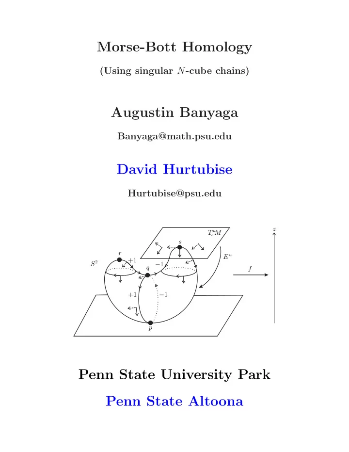
SLIDE 1 Morse-Bott Homology
(Using singular N-cube chains)
Augustin Banyaga
Banyaga@math.psu.edu
David Hurtubise
Hurtubise@psu.edu
f S z
2
p q r s T M
s u
E u ¡1 +1 +1 ¡1
Penn State University Park Penn State Altoona
SLIDE 2 The project
Construct a (singular) chain complex analogous to the Morse- Smale-Witten chain complex for Morse-Bott functions.
Question: Why would anyone want to do this?
After all, we can always perturb a smooth function to get a Morse-Smale
- function. Also, a Morse-Bott function determines a filtration, and
hence, a spectral sequence.
Example
If π : E → B is a smooth fiber bundle with fiber F, and f is a Morse function on B, then f ◦ π is a Morse-Bott function with critical submanifolds diffeomorphic to F. F
E
π
f
R
In particular, if G is a Lie group acting on M and π : EG → BG is the classifying bundle for G, then M
EG ×G M
π
f
R
So, this might be useful for studying equivariant homology: HG
∗ (M) = H∗(EG ×G M).
Other Examples: The square of the moment map, product structures in symplectic Floer homology, quantum cohomology, etc.
SLIDE 3 Perturbations
- 1. If f : M → R is a Morse-Bott function, study the Morse-
Smale-Witten complex as ε → 0 of h = f + ε
l
ρjfj .
- 2. If h : M → R is a Morse-Smale function, study the Morse-
Smale-Witten complex of εh : M → R as ε → 0.
SLIDE 4
Morse-Bott functions
Definition 1 A smooth function f : M → R on a smooth manifold M is called a Morse-Bott function if and only if Cr(f) is a disjoint union of connected submanifolds, and for each connected submanifold B ⊆ Cr(f) the normal Hessian is non-degenerate for all p ∈ B. Lemma 1 (Morse-Bott Lemma) Let f : M → R be a Morse-Bott function, and let B be a connected component of the critical set Cr(f). For any p ∈ B there is a local chart of M around p and a local splitting of the normal bundle of B ν∗(B) = ν+
∗ (B) ⊕ ν− ∗ (B)
identifying a point x ∈ M in its domain to (u, v, w) where u ∈ B, v ∈ ν+
∗ (B), w ∈ ν− ∗ (B) such that within this chart f
assumes the form f(x) = f(u, v, w) = f(B) + |v|2 − |w|2. Note that if p ∈ B, then this implies that TpM = TpB ⊕ ν+
p (B) ⊕ ν− p (B).
If we let λp = dim ν−
p (B) be the index of a connected critical
submanifold B, b = dim B, and λ∗
p = dim ν+ p (B), then we have
the fundamental relation m = b + λ∗
p + λp
where m = dim M.
SLIDE 5 Morse-Bott functions II
For p ∈ Cr(f) the stable manifold W s(p) and the unstable mani- fold W u(p) are defined the same as they are for a Morse function: W s(p) = {x ∈ M| lim
t→∞ ϕt(x) = p}
W u(p) = {x ∈ M| lim
t→−∞ ϕt(x) = p}.
Definition 2 If f : M → R is a Morse-Bott function, then the stable and unstable manifolds of a critical submanifold B are defined to be W s(B) =
W s(p) W u(B) =
W u(p). Theorem 1 (Stable/Unstable Manifold Theorem) The stable and unstable manifolds W s(B) and W u(B) are the sur- jective images of smooth injective immersions E+ : ν+
∗ (B) →
M and E− : ν−
∗ (B) → M. There are smooth endpoint maps
∂+ : W s(B) → B and ∂− : W u(B) → B given by ∂+(x) = limt→∞ ϕt(x) and ∂−(x) = limt→−∞ ϕt(x) which when restricted to a neighborhood of B have the structure of locally trivial fiber bundles.
SLIDE 6
Morse-Bott-Smale functions
Definition 3 (Morse-Bott-Smale Transversality) A func- tion f : M → R is said to satisfy the Morse-Bott-Smale transversality condition with respect to a given metric on M if and only if f is Morse-Bott and for any two connected crit- ical submanifolds B and B′, W u(p) intersects W s(B′) trans- versely, i.e. W u(p) ⋔ W s(B′), for all p ∈ B. Note: For a given Morse-Bott function f : M → R it may not be possible to pick a Riemannian metric for which f is Morse-Bott- Smale. Lemma 2 Suppose that B is of dimension b and index λB and that B′ is of dimension b′ and index λB′. Then we have the following where m = dim M: dim W u(B) = b + λB dim W s(B′) = b′ + λ∗
B′ = m − λB′
dim W(B, B′) = λB − λB′ + b (if W(B, B′) = ∅). Note: The dimension of W(B, B′) does not depend on the dimen- sion of the critical submanifold B′. This fact will be used when we define the boundary operator in the Morse-Bott-Smale chain complex.
SLIDE 7 The general form of a M-B-S complex
Assume that f : M → R is a Morse-Bott-Smale function and the manifold M, the critical submanifolds, and their negative nor- mal bundles are all orientable. Let Cp(Bi) be the group of “p- dimensional chains” in the critical submanifolds of index i. A Morse-Bott-Smale chain complex is of the form: ... . . . · · · C1(B2)
⊕ ∂0 ∂1
C2(B1)
⊕ ∂0 ∂1
⊕ ∂0 ∂1
⊕ ∂0
C3(B0)
⊕ ∂0 C2(B0) ⊕ ∂0 C1(B0) ⊕ ∂0 C0(B0) ⊕ ∂0 0
· · · C3(f)
C2(f)
C1(f)
C0(f)
where the boundary operator is defined as a sum of homomor- phisms ∂ = ∂0 ⊕ · · · ⊕ ∂m where ∂j : Cp(Bi) → Cp+j−1(Bi−j). This type of algebraic structure is known as a multicomplex. The homomorphism ∂0: For a deRham-type cohomology the-
- ry ∂0 = d. For a singular theory ∂0 = (−1)k∂, where ∂ is the
“usual” boundary operator from singular homology. Ways to define ∂1, . . . , ∂m:
- 1. deRham version: integration along the fiber.
- 2. singular versions: fibered product constructions.
SLIDE 8 The associated spectral sequence
The Morse-Bott chain multicomplex can be written as follows to resemble a first quadrant spectral sequence. . . . . . . . . . . . . C3(B0)
∂0
∂0
∂0
∂0
C2(B0)
∂0
∂0
∂0
∂0
C1(B0)
∂0
∂0
∂0
∂0
C0(B0) C0(B1)
∂1
∂1
∂1
More precisely, the Morse-Bott chain complex (C∗(f), ∂) is a fil- tered differential graded Z-module where the (increasing) filtration is determined by the Morse-Bott index. The associated bigraded module G(C∗(f)) is given by G(C∗(f))s,t = FsCs+t(f)/Fs−1Cs+t(f) ≈ Ct(Bs), and the E1 term of the associated spectral sequence is given by E1
s,t ≈ Hs+t(FsC∗(f)/Fs−1C∗(f))
where the homology is computed with respect to the boundary
- perator on the chain complex FsC∗(f)/Fs−1C∗(f) induced by
∂ = ∂0 ⊕ · · · ⊕ ∂m, i.e. ∂0.
SLIDE 9 The associated spectral sequence II
Since ∂0 = (−1)k∂, where ∂ is the “usual” boundary operator from singular homology, the E1 term of the spectral sequence is given by E1
s,t ≈ Hs+t(FsC∗(f)/Fs−1C∗(f)) ≈ Ht(Bs)
where Ht(Bs) denotes homology of the chain complex · · · ∂0 C3(Bs) ∂0 C2(Bs) ∂0 C1(Bs) ∂0 C0(Bs) ∂0 0. Hence, the E1 term of the spectral sequence is . . . . . . . . . . . . H3(B0) H3(B1)
d1
d1
d1
H2(B0) H2(B1)
d1
d1
d1
H1(B0) H1(B1)
d1
d1
d1
H0(B0) H0(B1)
d1
d1
d1
where d1 denotes the following connecting homomorphism of the triple (FsC∗(f), Fs−1C∗(f), Fs−2C∗(f). Hs+t(FsC∗(f)/Fs−1C∗(f))
d1
− → Hs+t−1(Fs−1C∗(f)/Fs−2C∗(f)) The differentials d0 and d1 in the spectral sequence are induced from the homomorphisms ∂0 and ∂1 in the multicomplex. How- ever, the differential dr for r ≥ 2 is, in general, not induced from the corresponding homomorphism ∂r in the multicomplex [J.M. Boardman, “Conditionally convergent spectral sequences”].
SLIDE 10 The Austin–Braam approach (∼1995)
(Modeled on deRham cohomology) Let Bi be the set of critical points of index i and Ci,j = Ωj(Bi) the set of j-forms on Bi. Austin and Braam define maps ∂r : Ci,j → Ci+r,j−r+1 for r = 0, 1, 2, . . . , m which raise the “total degree” i + j by one. . . . . . . . . . . . . Ω3(B0)
∂1 ∂2
∂1 ∂2
∂1 Ω3(B3)
· · · Ω2(B0)
∂0
∂2
∂0
∂2
∂0
∂0
Ω1(B0)
∂0
∂2
∂0
∂2
∂0
∂0
Ω0(B0)
∂0
∂0
∂0
∂0
Note: Note that the above diagram is not a double complex be- cause ∂2
1 = 0. However, it does determine a multicomplex [J.-P.
Meyer, “Acyclic models for multicomplexes”, Duke Math. J., 45 (1978), no. 1, p. 67–85; MR 0486489 (80b:55012)].)
SLIDE 11 The Austin–Braam cochain complex
The maps ∂r : Ωj(Bi) → Ωj−r+1(Bi+r) fit together to form a cochain complex where ∂ = ∂0 ⊕ · · · ⊕ ∂m and Ck(f) =
k
Ωk−i(Bi). Ω0(B3) Ω0(B2)
⊕
Ω0(B1)
Ω2(B1)
⊕
Ω0(B0)
Ω2(B0)
⊕
C0(f)
∂
∂
∂
Theorem 2 (Austin-Braam) For any j = 0, . . . , m
j
∂j−l∂j = 0. Hence, ∂2 = 0. Note: ∂2∂0 + ∂1∂1 + ∂0∂2 = 0. So, ∂2
1 = 0 in general.
Theorem 3 (Austin-Braam) H(C∗(f), ∂) ≈ H∗(M; R)
SLIDE 12 Compactified moduli spaces
For any two critical submanifolds B and B′ the flow ϕt induces an R-action on W u(B) ∩ W s(B′). Let M(B, B′) = (W u(B) ∩ W s(B′))/R be the quotient space of gradient flow lines from B to B′. Theorem 4 (Gluing) Suppose that B, B′, and B′′ are crit- ical submanifolds such that W u(B) ⋔ W s(B′) and W u(B′) ⋔ W s(B′′). In addition, assume that W u(x) ⋔ W s(B′′) for all x ∈ B′. Then for some ǫ > 0, there is an injective local diffeomorphism G : M(B, B′) ×B′ M(B′, B′′) × (0, ǫ) → M(B, B′′)
Theorem 5 (Compactification) Assume that f : M → R satisfies the Morse-Bott-Smale transversality condition. For any two distinct critical submanifolds B and B′ the moduli space M(B, B′) has a compactification M(B, B′), consisting
- f all the piecewise gradient flow lines from B to B′, which is
a compact smooth manifold with corners of dimension λB − λB′+b−1. Moreover, the beginning and endpoint maps extend to smooth maps ∂− : M(B, B′) → B ∂+ : M(B, B′) → B′, where ∂− has the structure of a locally trivial fiber bundle.
SLIDE 13 Integration along the fiber
Let π : E → B be a fiber bundle where B is a closed manifold, a typical fiber F is a compact oriented d-dimensional manifold with corners, and π∂ : ∂E → B is also a fiber bundle with fiber ∂F. A differential form on E may be written locally as π∗(φ)f(x, t)dti1 ∧ dti2 ∧ · · · ∧ dtir where φ is a form on B, x are coordinates on B, and the tj are coordinates on F. Definition 4 Integration along the fiber π∗ : Ωj(E) → Ωj−d(B) is defined by π∗(π∗(φ)f(x, t)dt1 ∧ dt2 ∧ · · · ∧ dtd) = φ
f(x, t)dt1 ∧ · · · ∧ dtd π∗(π∗(φ)f(x, t)dti1 ∧ dti2 ∧ · · · ∧ dtir) = 0 if r < d. The beginning point map ∂− : M(Bi+r, Bi) → Bi+r is such a fiber bundle and we can pullback along the endpoint map ∂+ : M(Bi+r, Bi) → Bi. Definition 5 Define ∂r : Ωj(Bi) → Ωj−r+1(Bi+r) by ∂r(ω) = dω r = 0 (−1)j(∂−)∗(∂∗
+ω) r = 0.
SLIDE 14 An example of Morse-Bott cohomology
Consider S2 = {(x, y, z) ∈ R3| x2 + y2 + z2 = 1}, and let f(x, y, z) = z2. Then B0 = E ≈ S1, B1 = ∅, and B2 = {n, s}.
S z 1 1 f
2 2
B0 B2 n s
R ⊕ R
⊕
Ω0(S1) d
- ∂1
- ≈
- Ω1(S1) d
- ∂2
- ⊕
- ≈
- ⊕
- ≈
- C0(f)
∂
C1(f)
∂
C2(f) ∂
ker d : Ω0(S1) → Ω1(S1) ≈ constant functions on S1 ≈ H0(S2; R) The map ∂2 : Ω1(S1) → R ⊕ R integrates a 1-form ω over the components of M(B2, B0) ≈ S1 ∐ S1, which have opposite orien-
∂2(ω) = (−1)(∂−)∗(∂∗
+ω) = (c, −c)
for some c ∈ R, and H2(C∗(f), ∂) ≈ R2/R ≈ R. If c = 0, then ω is in the image of d : Ω0(S1) → Ω1(S1), and hence H1(C∗(f), ∂) ≈ 0.
SLIDE 15 The Banyaga–Hurtubise approach (∼2007)
Modeled on cubical singular homology. Based on ideas from Austin and Braam (∼1995), Barraud and Cornea (∼2004), Fukaya (∼1995), Weber (∼2006) etc. Step 1: Generalize the notion of singular p-simplexes to allow maps from spaces other than the standard p-simplex △p ⊂ Rp+1
- r the unit p-cube Ip ⊂ Rp.
These generalizations of △p (or Ip) are called abstract topological chains, and the corresponding singular chains are called singular topological chains. Step 2: Show that the compactified moduli spaces of gradient flow lines are abstract topological chains, i.e. show that ∂0 is
- defined. Show that ∂0 extends to fibered products.
Step 3: Define the set of allowed domains Cp in the Morse- Bott-Smale chain complex as a collection of fibered products (with ∂0 defined) and show that the allowed domains are all compact
- riented smooth manifolds with corners.
Step 4: Define ∂1, . . . , ∂m using fibered products of compact- ified moduli spaces of gradient flow lines and the beginning and endpoint maps. Define ∂ = ∂0⊕· · ·⊕∂m and show that ∂ ◦∂ = 0. Step 5: Define orientation conventions on the elements of Cp and corresponding degeneracy relations to identify singular topological chains that are “essentially” the same. Show that ∂ = ∂0⊕· · ·⊕∂m is compatible with the degeneracy relations. Step 6: Show that the homology of the Morse-Bott-Smale chain complex (C∗(f), ∂∗) is independent of f : M → R.
SLIDE 16 The singular M-B-S chain complex
Let S∞
p (Bi) be the set of smooth singular Cp-chains in Bi (with re-
spect to the endpoint maps on moduli spaces), and let D∞
p (Bi) ⊆
S∞
p (Bi) be the subgroup of degenerate singular topological chains.
The chain complex ( ˜ C∗(f), ∂): S∞
0 (B2) ∂0
1 (B1) ⊕ ∂0 ∂1
0 (B1) ⊕ ∂0
2 (B0) ⊕ ∂0 S∞ 1 (B0) ⊕ ∂0 S∞ 0 (B0) ⊕ ∂0 0
˜ C2(f)
˜
C1(f)
˜
C0(f)
The Morse-Bott-Smale chain complex (C∗(f), ∂): S∞
0 (B2)/D∞ 0 (B2) ∂0
1 (B1)/D∞ 1 (B1) ⊕ ∂0
0 (B1)/D∞ 0 (B1) ⊕ ∂0
2 (B0)/D∞ 2 (B0) ⊕ ∂0 S∞ 1 (B0)/D∞ 1 (B0) ⊕ ∂0 S∞ 0 (B0)/D∞ 0 (B0) ⊕ ∂0 0
C2(f)
C1(f)
C0(f)
SLIDE 17 Step 1: Generalize the notion of singular p-simplexes to allow maps from spaces other than the standard p-simplex △p ⊂ Rp+1
- r the unit p-cube Ip ⊂ Rp.
For each integer p ≥ 0 fix a set Cp of topological spaces, and let Sp be the free abelian group generated by the elements of Cp, i.e. Sp = Z[Cp]. Set Sp = {0} if p < 0 or Cp = ∅. Definition 6 A boundary operator on the collection S∗ of groups {Sp} is a homomorphism ∂p : Sp → Sp−1 such that
- 1. For p ≥ 1 and P ∈ Cp ⊆ Sp, ∂p(P) =
k nkPk where
nk = ±1 and Pk ∈ Cp−1 is a subspace of P for all k.
- 2. ∂p−1 ◦ ∂p : Sp → Sp−2 is zero.
We call (S∗, ∂∗) a chain complex of abstract topological chains. Elements of Sp are called abstract topological chains of degree p. Definition 7 Let B be a topological space and p ∈ Z+. A singular Cp-space in B is a continuous map σ : P → B where P ∈ Cp, and the singular Cp-chain group Sp(B) is the free abelian group generated by the singular Cp-spaces. Define Sp(B) = {0} if Sp = {0} or B = ∅. Elements of Sp(B) are called singular topological chains of degree p. Note: These definitions are quite general. To construct the M-B-S chain complex we really only need Cp to include the p-dimensional faces of an N-cube, the compactified moduli spaces of gradient flow lines of dimension p, and the components of their fibered products
SLIDE 18 For p ≥ 1 there is a boundary operator ∂p : Sp(B) → Sp−1(B) induced from the boundary operator ∂p : Sp → Sp−1. If σ : P → B is a singular Cp-space in B, then ∂p(σ) is given by the formula ∂p(σ) =
nkσ|Pk where ∂p(P) =
nkPk. The pair (S∗(B), ∂∗) is called a chain complex of singular topolog- ical chains in B. Singular N-cube chains Pick some large positive integer N and let IN = {(x1, . . . , xN) ∈ RN| 0 ≤ xj ≤ 1, j = 1, . . . , N} denote the unit N-cube. For every 0 ≤ p ≤ N let Cp be the set consisting of the faces of IN
- f dimension p, i.e. subsets of IN where p of the coordinates are
free and the rest of the coordinates are fixed to be either 0 or 1. For every 0 ≤ p ≤ N let Sp be the free abelian group generated by the elements of Cp. For P ∈ Cp we define ∂p(P) =
p
(−1)j P|xj=1 − P|xj=0
where xj denotes the jth free coordinate of P.
SLIDE 19 Singular cubical boundary operator (Massey)
B
¾ B1 A1
I
1 2
I
A2 B2
The chain σ : I2 → B has boundary ∂2(σ) = (−1)[σ ◦ A1 − σ ◦ B1] + [σ ◦ A2 − σ ◦ B2] where the terms in the sum are all maps with domain I1 = [0, 1]. Topological cubical boundary operator (B–H)
I
2
@ =
A1 A2 B2 B1 A1 A2 B2
¡ ¡
+ B1
( 1)
¡
The chain σ : I2 → B has boundary ∂2(σ) = (−1)[σ|A1 − σ|B1] + [σ|A2 − σ|B2] and the degeneracy relations identify terms that are “essentially” the same.
SLIDE 20 Recovering singular homology (degeneracy relations) A continuous map σP : P → B from a p-face P of IN into a topological space B is a singular Cp-space in B. The boundary
∂p(σP) =
p
(−1)j σP|xj=1 − σP|xj=0
where σP|xj=0 denotes the restriction σP : P|xj=0 → B and σP|xj=1 denotes the restriction σP : P|xj=1 → B. Definition 8 Let σP and σQ be singular Cp-spaces in B and let ∂p(Q) =
j njQj ∈ Sp−1. For any map α : P → Q, let
∂p(σQ)◦α denote the formal sum
j nj(σQ ◦α)|α−1(Qj). Define
the subgroup Dp(B) ⊆ Sp(B) of degenerate singular N-cube chains to be the subgroup generated by the following elements.
- 1. If α is an orientation preserving homeomorphism such that
σQ◦α = σP and ∂p(σQ)◦α = ∂p(σP), then σP −σQ ∈ Dp(B).
- 2. If σP does not depend on some free coordinate of P, then
σP ∈ Dp(B). Theorem 6 The boundary operator for singular N-cube chains ∂p : Sp(B) → Sp−1(B) descends to a homomorphism ∂p : Sp(B)/Dp(B) → Sp−1(B)/Dp−1(B), and Hp(S∗(B)/D∗(B), ∂∗) ≈ Hp(B; Z) for all p < N.
SLIDE 21 Step 2: Show that the compactified moduli spaces of gradient flow lines are abstract topological chains, i.e. show that ∂0 is
- defined. Show that ∂0 extends to fibered products.
Fibered products Suppose that σ1 : P1 → B is a singular Sp1-space and σ2 : P2 → B is a singular Sp2-space where (S∗, ∂∗) is a chain complex of abstract topological chains. The fibered product of σ1 and σ2 is P1 ×B P2 = {(x1, x2) ∈ P1 × P2| σ1(x1) = σ2(x2)}. This construction extends linearly to singular topological chains. Definition 9 The degree of the fibered product P1 ×B P2 is defined to be p1 +p2 −b. The boundary operator applied to the fibered product is defined to be ∂(P1 ×B P2) = ∂P1 ×B P2 + (−1)p1+bP1 ×B ∂P2 where ∂P1 and ∂P2 denote the boundary operator applied to the abstract topological chains P1 and P2. If σ1 = 0, then we define 0 ×B P2 = 0. Similarly, if σ2 = 0, then P1 ×B 0 = 0. Lemma 3 The fibered product of two singular topological chains is an abstract topological chain, i.e. the boundary operator on fibered products is of degree -1 and satisfies ∂ ◦ ∂ = 0. More-
- ver, the boundary operator on fibered products is associative,
i.e. ∂((P1 ×B1 P2) ×B2 P3) = ∂(P1 ×B1 (P2 ×B2 P3)).
SLIDE 22 Proof that P1 ×B P2 is an abstract topological chain The degree of P1 ×B P2 is p1 + p2 − b. Since ∂ is a boundary operator on P1 and P2, the degree of ∂P1 is p1 − 1 and the degree of ∂P2 is p2 − 1. Hence both ∂P1 ×B P2 and P1 ×B ∂P2 have degree p1 + p2 − b − 1. To see that ∂2(P1 ×B P2) = 0 we compute as follows. ∂(∂(P1 ×B P2)) = ∂(∂P1 ×B P2 + (−1)p1+bP1 ×B ∂P2) = ∂2P1 ×B P2 + (−1)p1−1+b∂P1 ×B ∂P2 + (−1)p1+b(∂P1 ×B ∂P2 + (−1)p1+bP1 ×B ∂2P2) = 0. Associativity Given the data of a triple P1
σ11 B1
P2
σ12
P3
σ23
- we can form the iterated fibered product (P1 ×B1 P2)×B2 P3 using
σ23 and the map σ22◦π2 : P1×B1P2 → B2, where π2 : P1×B1P2 → P2 denotes projection to the second component. That is, we have the following diagram. (P1 ×B1 P2) ×B2 P3
π1
σ23
π1
σ12
P1
σ11
B1
SLIDE 23 Compactified moduli spaces and ∂0 Definition 10 Let Bi be the set of critical points of index i. For any j = 1, . . . , i we define the degree of M(Bi, Bi−j) to be j + bi − 1 and the boundary operator to be ∂M(Bi, Bi−j) = (−1)i+bi
M(Bi, Bn) ×Bn M(Bn, Bi−j) where bi = dim Bi and the fibered product is taken over the beginning and endpoint maps ∂− and ∂+. If Bn = ∅, then M(Bi, Bn) = M(Bn, Bi−j) = 0. Lemma 4 The degree and boundary operator for M(Bi, Bi−j) satisfy the axioms for abstract topological chains, i.e. the boundary operator on the compactified moduli spaces is of de- gree −1 and ∂ ◦ ∂ = 0.
Proof: Let d = deg M(Bi, Bn) = i − n + bi − 1. Then ∂(M(Bi, Bn) ×Bn M(Bn, Bi−j)) = ∂M(Bi, Bn) ×Bn M(Bn, Bi−j) + (−1)d+bnM(Bi, Bn) ×Bn ∂M(Bn, Bi−j) = (−1)i+bi
n<s<i
M(Bi, Bs, Bn, Bi−j) + (−1)i+bi−1
M(Bi, Bn, Bt, Bi−j) Therefore, ∂2M(Bi, Bi−j) = (−1)i+bi
i−j<n<i
n<s<i
M(Bi, Bs, Bn, Bi−j)+ (−1)i+bi−1
M(Bi, Bn, Bt, Bi−j)
(−1)i+bi
M(Bi, Bs, Bn, Bi−j)+ (−1)i+bi−1
M(Bi, Bn, Bt, Bi−j)
✷
SLIDE 24 Step 3: Define the set of allowed domains Cp in the Morse- Bott-Smale chain complex as a collection of fibered products (with ∂0 defined) and show that the allowed domains are all compact
- riented smooth manifolds with corners.
For any p ≥ 0 let Cp be the set consisting of the faces of IN of dimension p and the connected components of degree p of fibered products of the form Q×Bi1M(Bi1, Bi2)×Bi2M(Bi2, Bi3)×Bi3· · ·×Bin−1M(Bin−1, Bin) where m ≥ i1 > i2 > · · · > in ≥ 0, Q is a face of IN of dimension q ≤ p, σ : Q → Bi1 is smooth, and the fibered products are taken with respect to σ and the beginning and endpoint maps. Theorem 7 The elements of Cp are compact oriented smooth manifolds with corners, and there is a boundary operator ∂ : Sp → Sp−1 where Sp is the free abelian group generated by the elements
Let S∞
p (Bi) denote the subgroup of the singular Cp-chain group
Sp(Bi) generated by those maps σ : P → Bi that satisfy the following two conditions:
- 1. The map σ is smooth.
- 2. If P ∈ Cp is a connected component of a fibered product,
then σ = ∂+ ◦ π, where π denotes projection onto the last component of the fibered product. Define ∂0 : S∞
p (Bi) → S∞ p−1(Bi) by ∂0 = (−1)p+i∂.
SLIDE 25
Step 4: Define ∂1, . . . , ∂m using fibered products of compact- ified moduli spaces of gradient flow lines and the beginning and endpoint maps. Define ∂ = ∂0⊕· · ·⊕∂m and show that ∂ ◦∂ = 0. If σ : P → Bi is a singular Cp-space in S∞
p (Bi), then for any
j = 1, . . . , i composing the projection map π2 onto the second component of P ×Bi M(Bi, Bi−j) with the endpoint map ∂+ : M(Bi, Bi−j) → Bi−j gives a map P ×Bi M(Bi, Bi−j)
π2
− → M(Bi, Bi−j)
∂+
− → Bi−j. The next lemma shows that restricting this map to the connected components of the fibered product P ×BiM(Bi, Bi−j) and adding these restrictions (with the sign determined by the orientation when the dimension of a component is zero) defines an element ∂j(σ) ∈ S∞
p+j−1(Bi−j).
Lemma 5 If σ : P → Bi is a singular Cp-space in S∞
p (Bi),
then for any j = 1, . . . , i adding the components of P ×Bi M(Bi, Bi−j) (with sign when the dimension of a component is zero) yields an abstract topological chain of degree p + j − 1. That is, we can identify P ×Bi M(Bi, Bi−j) ∈ Sp+j−1. Thus, for all j = 1, . . . , i there is an induced homomorphism ∂j : S∞
p (Bi) → S∞ p+j−1(Bi−j)
which decreases the Morse-Bott degree p + i by 1.
SLIDE 26 Proposition 1 For every j = 0, . . . , m
j
∂q∂j−q = 0. Proof: When q = 0 we compute as follows. ∂0(∂j(P)) = ∂0
- P ×Bi M(Bi, Bi−j)
- = (−1)p+i−1
∂P ×Bi M(Bi, Bi−j) + (−1)p+biP ×Bi ∂M(Bi, Bi−j)
- = (−1)p+i−1∂P ×Bi M(Bi, Bi−j) +
(−1)2p+2bi+2i−1
P ×Bi M(Bi, Bn) ×Bn M(Bn, Bi−j) If 1 ≤ q ≤ j − 1, then ∂q(∂j−q(P)) = P ×Bi M(Bi, Bi−j+q) ×Bi−j+q M(Bi−j+q, Bi−j) and if q = j, then ∂j(∂0(P)) = (−1)p+i∂P ×Bi M(Bi, Bi−j). Summing these expressions gives the desired result. ✷ Corollary 1 The pair ( ˜ C∗(f), ∂) is a chain complex, i.e. ∂ ◦ ∂ = 0.
SLIDE 27 Step 5: Define orientation conventions on the elements of Cp and corresponding degeneracy relations to identify singular topological chains that are “essentially” the same. Show that ∂ = ∂0⊕· · ·⊕∂m is compatible with the degeneracy relations.
Definition 11 (Degeneracy Relations for the Morse-Bott-Smale Chain Complex) Let σP, σQ ∈ S∞
p (Bi) be singular Cp-spaces in Bi and let ∂Q = j njQj ∈ Sp−1. For any
map α : P → Q, let ∂0σQ ◦α denote the formal sum (−1)p+i
j nj(σQ ◦α)|α−1(Qj). Define
the subgroup D∞
p (Bi) ⊆ S∞ p (Bi) of degenerate singular topological chains to be the
subgroup generated by the following elements.
- 1. If α is an orientation preserving homeomorphism such that σQ ◦ α = σP and ∂0σQ ◦
α = ∂0σP, then σP − σQ ∈ D∞
p (Bi).
- 2. If P is a face of IN and σP does not depend on some free coordinate of P, then
σP ∈ D∞
p (Bi) and ∂j(σP) ∈ D∞ p+j−1(Bi−j) for all j = 1, . . . , m.
- 3. If P and Q are connected components of some fibered products and α is an orientation
reversing map such that σQ ◦ α = σP and ∂0σQ ◦ α = ∂0σP, then σP + σQ ∈ D∞
p (Bi).
- 4. If Q is a face of IN and R is a connected component of a fibered product
Q ×Bi1 M(Bi1, Bi2) ×Bi2 M(Bi2, Bi3) ×Bi3 · · · ×Bin−1 M(Bin−1, Bin) such that deg R > dim Bin, then σR ∈ D∞
r (Bin) and ∂j(σR) ∈ D∞ r+j−1(Bin−j) for all
j = 0, . . . , m.
α nασα ∈ S∗(R) is a smooth singular chain in a connected component R of a
fibered product (as in (4)) that represents the fundamental class of R and (−1)r+in∂0σR −
nα∂(σR ◦ σα) is in the group generated by the elements satisfying one of the above conditions, then σR −
nα(σR ◦ σα) ∈ D∞
r (Bin)
and ∂j
nα(σR ◦ σα)
r+j−1(Bin−j)
for all j = 1, . . . , m.
SLIDE 28
Step 6: Show that the homology of the Morse-Bott-Smale chain complex (C∗(f), ∂∗) is independent of f : M → R. Given two Morse-Bott-Smale functions f1, f2 : M → R we pick a smooth function F21 : M × R → R meeting certain transversality requirements such that lim
t→−∞ F21(x, t) = f1(x) + 1
lim
t→+∞ F21(x, t) = f2(x) − 1
for all x ∈ M. The compactified moduli spaces of gradient flow lines of F21 (the time dependent gradient flow lines) are used to define a chain map (F21)✷ : C∗(f1) → C∗(f2), where (C∗(fk), ∂) is the Morse-Bott chain complex of fk for k = 1, 2. Next we consider the case where we have four Morse-Bott-Smale functions fk : M → R where k = 1, 2, 3, 4, and we pick a smooth function H : M × R × R → R meeting certain transversality requirements such that lim
s→−∞ lim t→−∞ H(x, s, t) = f1(x) + 2
lim
s→+∞ lim t→−∞ H(x, s, t) = f2(x)
lim
s→−∞ lim t→+∞ H(x, s, t) = f3(x)
lim
s→+∞ lim t→+∞ H(x, s, t) = f4(x) − 2
for all x ∈ M.
SLIDE 29 H f = H f = + 2 H f =
1 3 4 2
H f = 2 ¡ s t
The compactified moduli spaces of gradient flow lines of H are used to define a chain homotopy between (F43)✷ ◦ (F31)✷ and (F42)✷ ◦ (F21)✷ where (Flk)✷ : C∗(fk) → C∗(fl) is the map de- fined above for k, l = 1, 2, 3, 4. In homology the map (Fkk)∗ : H∗(C∗(fk), ∂) → H∗(C∗(fk), ∂) is the identity for all k, and hence (F12)∗ ◦ (F21)∗ = (F11)∗ ◦ (F11)∗ = id (F21)∗ ◦ (F12)∗ = (F22)∗ ◦ (F22)∗ = id. Therefore, (F21)∗ : H∗(C∗(f1), ∂) → H∗(C∗(f2), ∂) is an isomorphism. Theorem 8 (Morse-Bott Homology Theorem) The ho- mology of the Morse-Bott chain complex (C∗(f), ∂) is indepen- dent of the Morse-Bott-Smale function f : M → R. There- fore, H∗(C∗(f), ∂) ≈ H∗(M; Z).
SLIDE 30 An example of Morse-Bott homology
Consider M = S2 = {(x, y, z) ∈ R3| x2 + y2 + z2 = 1}, and let f(x, y, z) = z2. Then B0 ≈ S1, B1 = ∅, and B2 = {n, s}.
S z 1 1 f
2 2
B0 B2 n s
The degeneracy conditions imply S∞
0 (B2)/D∞ 0 (B2) ≈< n, s >≈ Z ⊕ Z,
and S∞
p (B2)/D∞ p (B2) = 0 for p > 0.
< n, s >
∂0
∂0
∂0
2 (B0)/D∞ 2 (B0) ⊕ ∂0 S∞ 1 (B0)/D∞ 1 (B0) ⊕ ∂0 S∞ 0 (B0)/D∞ 0 (B0) ⊕ ∂0 0
C2(f)
C1(f)
C0(f)
The group S∞
k (B0)/D∞ k (B0) is non-trivial for all k ≤ N, but
Hk(C∗(f), ∂) = 0 if k > 2 and ∂0 : S∞
3 (B0)/D∞ 3 (B0) →
S∞
2 (B0)/D∞ 2 (B0) maps onto the kernel of the boundary operator
∂0 : S∞
2 (B0)/D∞ 2 (B0) → S∞ 1 (B0)/D∞ 1 (B0) because the bottom
row in the above diagram computes the smooth integral singular homology of B0 ≈ S1.
SLIDE 31 The moduli space M(B2, B0) is a disjoint union of two copies of S1 with opposite orientations. This moduli space can be viewed as a subset of the manifold S2 since M(B2, B0) = M(B2, B0).
S2 n s M(B ,B )
2
@+ n£ M(B ,B )
2
s£ M(B ,B )
2 B
2 2
B
There is an orientation reversing map α : n ×n M(B2, B0) → s ×s M(B2, B0) such that ∂2(n) ◦ α = ∂2(s). Since ∂0(∂2(n)) = ∂0(∂2(s)) = 0, the degeneracy conditions imply that ∂2(n + s) = ∂2(n) + ∂2(s) = 0 ∈ S1(B0)/D1(B0). They also imply that ∂2 maps either n or s onto a representative
ker ∂0 : S∞
1 (B0)/D∞ 1 (B0) → S∞ 0 (B0)/D∞ 0 (B0)
im ∂0 : S∞
2 (B0)/D∞ 2 (B0) → S∞ 1 (B0)/D∞ 1 (B0) ≈ H1(S1; Z) ≈ Z
depending on the orientation chosen for B0. Therefore, Hk(C∗(f), ∂) =
0 otherwise.
SLIDE 32 References
- D.M. Austin and P.J. Braam, Morse-Bott theory and equiv-
ariant cohomology, The Floer memorial volume, 123–183,
- Progr. Math., 133, Birkhuser, Basel, 1995. MR1362827
- J.-F. Barraud and O. Cornea, Lagrangian intersections and
the Serre spectral sequence, arXiv:math DG/0404094 (2004).
- U. Frauenfelder, The Arnold-Givental conjecture and mo-
ment Floer homology, Int. Math. Res. Not. (2004), no. 42, 2179–2269. MR2076142
- K. Fukaya, Floer homology of connected sum of homology
3-spheres, Topology 35 (1996), no. 1, 89–136. MR1367277
- H. Hofer, K. Wysocki, and E. Zehnder, A General Fredholm
Theory I and II, arXiv:math FA/0612604v2 and arXiv:math FA/0705.1310v1 (2007).
- J. Latschev, Gradient flows of Morse-Bott functions, Math.
- Ann. 318 (2000), no. 4, 731–759. MR1802508
- G. Liu and G. Tian, On the equivalence of multiplicative
structures in Floer homology and quantum homology, Acta
- Math. Sin. (Engl. Ser.) 15 (1999), no. 1, 53–80. MR1701133
- Y. Ruan and G. Tian, Bott-type symplectic Floer cohomol-
- gy and its multiplication structures, Math. Res. Lett. 2
(1995), no. 2, 203–219. MR1324703
- J. Weber, The Morse-Witten complex via dynamical sys-
tems, Expo. Math. 24 (2006), 127–159. MR722297
SLIDE 33 Examples with fibered products
Fibered products of simplicial complexes Let f : [0, 1] → [0, 1] × [−1, 1] be given by f(t) =
- (t, e−1/t2 sin(π/t)) if t = 0
(0, 0) if t = 0 and g : [0, 1]×[0, 1] → [0, 1]×[−1, 1] be given by g(x, y) = (x, 0). Then f and g are maps between finite simplicial complexes whose fibered product [0, 1] ×(f,g) [0, 1] × [0, 1] = {(t, t, 0) ∈ [0, 1] × [0, 1] × [0, 1]| t = 0, 1, 1/2, 1/3, . . .} is not a finite simplicial complex. Perturbations and fibered products
Anon-transverse pointofintersection Nointersectionpoints Onetransverse pointofintersection Twotransverse pointsofintersections
If f : P1 → B and g : P2 → B do not meet transversally, and we perturb f to ˜ f : P1 → B so that ˜ f and g do meet transversally, then the fibered product P1 ×( ˜
f,g) P2
might depend on the perturbation.
SLIDE 34 Triangulations and fibered products Having triangulations on two spaces does not immediately induce a triangulation on the fibered product. In fact, there are simple diagrams of polyhedra and piecewise linear maps for which the diagram is not triangulable: R
g
← P
f
→ Q There may not exist triangulations of P, Q, and R with respect to which both f and g are simplicial. [J.L. Bryant, Triangulation and general position of PL diagrams, Top. App. 34 (1990), 211-233] The Banyaga-Hurtubise approach
- 1. Work in the category of compact smooth manifolds with cor-
ners instead of the category of finite simplicial complexes.
- 2. They prove that all of the relevant fibered products are com-
pact smooth manifolds with corners.
- 3. They prove that it is not necessary to perturb the beginning
and endpoint maps to achieve transversality. So, they don’t have to worry about the fibered products changing under per- turbations.
- 4. They don’t have to deal with any issues involving triangu-
lations because their approach allows singular chains whose domains are spaces more general than a simplex.