Morceaux choisis It is often said that 80% of data analysis is - - PowerPoint PPT Presentation

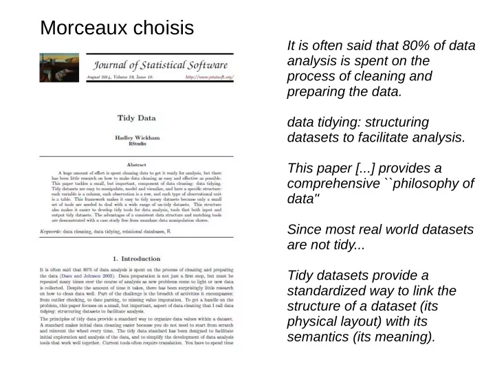
It is often said that 80% of data analysis is spent on the process of cleaning and preparing the data. data tidying: structuring datasets to facilitate analysis. This paper [...] provides a comprehensive ``philosophy of data'' Since most real world datasets are not tidy... Tidy datasets provide a standardized way to link the structure of a dataset (its physical layout) with its semantics (its meaning).

Morceaux choisis

http://hadley.nz/

http://hadley.nz/

http://ggplot2.org/ http://ggplot2.org/resources/2007-past-present-future.pdf http://ggplot2.org/resources/2007-vanderbilt.pdf http://docs.ggplot2.org/current/ https://www.youtube.com/results?search_query=hadley+wicham

tidyr Data cleaunp dplyr Data handling ggpot2 Data Visualization

Like families, tidy datasets are all alike but every messy dataset is messy in its own way.

« Les familles heureuses se ressemblent toutes. Les familles malheureuses sont malheureuses chacune à leur manière. »

https://deselection.wordpress.com/2010/11/12/le-principe-danna-karenine/

Le principe d'Anna Karenine

En d’autres termes, le succès demande que plusieurs conditions soient réunies. Une seule condition manquée est suffisante pour conduire à l’échec.

Much earlier, Aristotle states the same principle in the Nichomachean Ethics (Book 2): Again, it is possible to fail in many ways (for evil belongs to the class of the unlimited, as the Pythagoreans conjectured, and good to that of the limited), while to succeed is possible only in

• ne way (for which reason also one is easy and

the other difficult – to miss the mark easy, to hit it difficult); for these reasons also, then, excess and defect are characteristic of vice, and the mean of virtue; For men are good in but one way, but bad in many.

Version Aristote

https://en.wikipedia.org/wiki/Anna_Karenina_principle

• ∀x P(x) se lit « pour tout x P(x) » et signifie « tout objet du domaine

considéré possède la propriété P »

• ∃x P(x) signifie il existe au moins un x tel que P(x) (un objet au moins du

domaine considéré possède la propriété P)

Négation des quantificateurs La négation de x P(x) est : ∃

¬ x P(x), soit :

∃

x ∀ ¬P(x)

La négation de ∀x P(x) est : ¬∀x P(x), soit : ∃x ¬P(x)

https://fr.wikipedia.org/wiki/Quantificateur_(logique)

Logique : quantificateurs universel et existentiel

Logique classique

• Le tiers exclu énonce que pour toute proposition mathématique considérée, elle-même ou sa négation

est vraie : A ∨ ¬A

• Le raisonnement par l'absurde : ¬¬ A ⇒ A
• La contraposition : (¬Β ⇒ ¬A) ⇒ (A ⇒ B)
• L'implication matérielle : (Α ⇒ B) ⇔ (¬Α ∨ B)

https://fr.wikipedia.org/wiki/Logique_classique

H0 : toutes les moyennes sont égales H1 : non H0 Si rejet de H0, on sait qu'au moins une moyenne est différente des autres, mais laquelle ? → test post-hoc

ANOVA

https://fr.wikipedia.org/wiki/Analyse_de_la_variance

Ils sont tous égaux ! Ils ne sont pas tous égaux ! → Ils sont tous différents Ils ne sont pas tous égaux ! → un seul est différent des autres

messy tidy

Le terme tidy fait référence à une façon optimale (?) de présenter les données pour une analyse statistique. Une version messy peut être préférable pour une meilleure lisibilité des données.

Dans une publi, cette version ↑, plus compacte, est peut-etre préférable. Mais : impression d'avoir affaire à une table de contingence → test de chi2...

Tidy data

messy tidy

Tidy data

• 1. Each variable forms a column.
• 2. Each observation forms a row.
• 3. Each type of observational unit

forms a table.

Messy data is any other arrangement of the data.

Messy data

• Column headers are values, not variable names.
• Multiple variables are stored in one column.
• Variables are stored in both rows and columns.
• Multiple types of observational units are stored in the

same table.

• A single observational unit is stored in multiple tables.

Real datasets can, and often do, violate the three precepts of tidy data in almost every way

• imaginable. While occasionally you do get a dataset

that you can start analyzing immediately, this is the exception, not the rule. This section describes the five most common problems with messy datasets, along with their remedies:

Surprisingly, most messy datasets, including types of messiness not explicitly described above, can be tidied with a small set of tools: melting, string splitting, and casting.

Column headers are values, not variable names

3 variables :

• religion
• revenu
• effectif

... Chaque colonne représente une variable ; chaque ligne, une

• bservation

Tidying when column headers are values: melting

Columns corresponds to RNAseq data of different conditions (B, C, D) and 3 biological replicates ⇒ Wide dataset = natural initial format, nice format to summarise the data but not so nice to model or to plot melt() function allows to turn columns into rows ⇒ Molten datset is a nice format for models across times for example

Variables are stored in both rows and columns

Cette colonne contient un nom de variable ! Une variable par colonne, une

• bservation par ligne

Tidying when multiple variables are stored in one column: casting

Casting changes rows into columns (inverse of melting) Values of the 2 variables tmax and tmin are recorded in the same column but on 2 rows After casting the 2 variables are recorded in 2 columns

Tidying when …

• Variables are stored in both rows and columns: combination of

melting and casting

• Multiple types in one table (e.g. values collected at multiple

levels needed in the same table): merging

• One type in multiple tables : plyr package helps to read a list
• f file (ldplyr)

Tidy tools 1) Manipulation 2) Visualisation 3) Modélisation

• Filter: subsetting or removing observations based on some

condition.

• Transform: adding or modifying variables. These modications

can involve either a single variable (e.g., log-transformation), or multiple variables (e.g., computing density from weight and volume).

• Aggregate: collapsing multiple values into a single value (e.g.,

by summing or taking means).

• Sort: changing the order of observations.

Manipulation

All these operations are made easier when there is a consistent way to refer to variables. Tidy data provides this because each variable resides in its own column. Ensure input and output-tidiness

plyr,dplyr packages

Visualisation

Tidy visualization tools only need to be input-tidy as their

• utput is visual.

It provides a comprehensive ''philosophy of data": one that underlies my work in the plyr (Wickham 2011) and ggplot2 (Wickham 2009) packages.

ggplot2 package

Logique ggplot2 : syntaxe adaptée à un input tidy.

Source: http://ggplot2.org/resources/2007-past-present-future.pdf Hadley Wicham dixit:

str(mtcars) 'data.frame': 32 obs. of 11 variables: $ mpg : num 21 21 22.8 21.4 18.7 18.1 14.3 24.4 22.8 19.2 ... $ cyl : num 6 6 4 6 8 6 8 4 4 6 ... $ disp: num 160 160 108 258 360 ... $ hp : num 110 110 93 110 175 105 245 62 95 123 ... $ drat: num 3.9 3.9 3.85 3.08 3.15 2.76 3.21 3.69 3.92 3.92 ... $ wt : num 2.62 2.88 2.32 3.21 3.44 ... $ qsec: num 16.5 17 18.6 19.4 17 ... $ vs : num 0 0 1 1 0 1 0 1 1 1 ... $ am : num 1 1 1 0 0 0 0 0 0 0 ... $ gear: num 4 4 4 3 3 3 3 4 4 4 ... $ carb: num 4 4 1 1 2 1 4 2 2 4 ... head (mtcars) mpg cyl disp hp drat wt qsec vs am gear carb Mazda RX4 21.0 6 160 110 3.90 2.620 16.46 0 1 4 4 Mazda RX4 Wag 21.0 6 160 110 3.90 2.875 17.02 0 1 4 4 Datsun 710 22.8 4 108 93 3.85 2.320 18.61 1 1 4 1 Hornet 4 Drive 21.4 6 258 110 3.08 3.215 19.44 1 0 3 1 Hornet Sportabout 18.7 8 360 175 3.15 3.440 17.02 0 0 3 2 Valiant 18.1 6 225 105 2.76 3.460 20.22 1 0 3 1

ggplot(mtcars, aes(x=mpg,y=hp)) + geom_point() + geom_point(aes(colour = cyl, size=carb, shape=factor(gear))) plot(mtcars$mpg,mtcars$hp, col=mtcars$cyl-3, pch=mtcars$gear+15, cex=mtcars$carb/3)

toto=mtcars colnames(toto)=NULL plot(toto[,1],toto[,4], col=toto[,2]-3, pch=toto[,10]+15, cex=toto[,11]/3)cex=mtcars $carb/3)

toto=mtcars colnames(toto)=NULL plot(toto[,1],toto[,4], col=toto[,2]-3, pch=toto[,10]+15, cex=toto[,11]/3)cex=mtcars $carb/3) ggplot(toto, aes(x=toto[,1],y=toto[,4])) geom_point() + geom_point(aes(colour = toto[,2], size=toto[,11], shape=factor(toto[,10]))) Error in geom_point() geom_point(aes(colour = toto[, 2], size = toto[, : non-numeric argument to binary operator

scaled <- as.data.frame(lapply(mtcars, ggplot2:::rescale01)) scaled$model <- rownames(mtcars) # add model names as a variable mtcarsm <- reshape2::melt(scaled) filter(mtcarsm,model=="Lotus Europa") model variable value 1 Lotus Europa mpg 0.8510638 2 Lotus Europa cyl 0.0000000 3 Lotus Europa disp 0.0598653 4 Lotus Europa hp 0.2155477 5 Lotus Europa drat 0.4654378 6 Lotus Europa wt 0.0000000 7 Lotus Europa qsec 0.2857143 8 Lotus Europa vs 1.0000000 9 Lotus Europa am 1.0000000 10 Lotus Europa gear 1.0000000 11 Lotus Europa carb 0.1428571

ggplot(mtcarsm, aes(x = variable, y = value))

ggplot(mtcarsm, aes(x = variable, y = value)) + geom_line(aes(group = model, color = model), size = 2) +

ggplot(mtcarsm, aes(x = variable, y = value)) + geom_line(aes(group = model, color = model), size = 2) + theme(strip.text.x = element_text(size = rel(0.8)), axis.text.x = element_blank(), axis.ticks.y = element_blank(), axis.text.y = element_blank())

ggplot(mtcarsm, aes(x = variable, y = value)) + geom_line(aes(group = model, color = model), size = 2) + theme(strip.text.x = element_text(size = rel(0.8)), axis.text.x = element_blank(), axis.ticks.y = element_blank(), axis.text.y = element_blank()) + guides(color = "none")

ggplot(mtcarsm, aes(x = variable, y = value)) + geom_line(aes(group = model, color = model), size = 2) + theme(strip.text.x = element_text(size = rel(0.8)), axis.text.x = element_blank(), axis.ticks.y = element_blank(), axis.text.y = element_blank()) + guides(color = "none") + facet_wrap(~ model)

Modelisation

Modeling is the driving inspiration of this work because most modeling tools work best with tidy datasets. Every statistical language has a way of describing a model as a connection among different variables, a domain specic language that connects responses to predictors

Conclusion

Apart from tidying, there are many other tasks involved in cleaning data: parsing dates and numbers, identifying missing values, correcting character encodings (for international data), matching similar but not identical values (created by typos), verifying experimental design, and filling in structural missing values, not to mention model-based data cleaning that identifies suspicious values. Can we develop other frameworks to make these tasks easier?

Les éléments mentionnés ci-dessus sont intimement liées aux utilisations croisées d'un logiciel de statistique et d'un tableur : plusieurs onglets, cellules fusionnées, format de dates, ouverture par défaut des fichiers csv...

• Introduction aux langages, à l’architecture des machines

et au calcul

• R, histoire et écosystème
• R avancé (dplyr, fonctions, environnements…)
• Calcul parallèle avec R
• Débogage et profilage de code R
• Systèmes de gestion de version
• Développement de packages R
• Visualisation de données