SLIDE 1
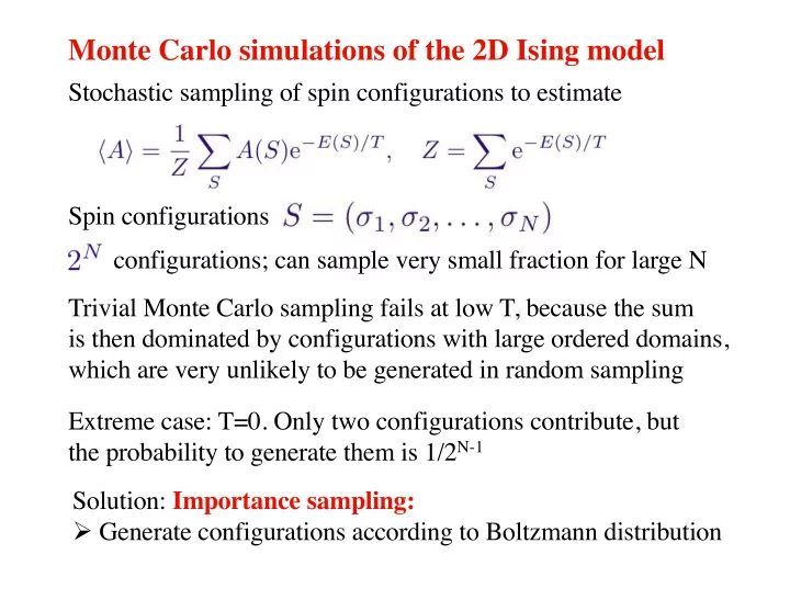
Monte Carlo simulations of the 2D Ising model
Stochastic sampling of spin configurations to estimate Spin configurations configurations; can sample very small fraction for large N Trivial Monte Carlo sampling fails at low T, because the sum is then dominated by configurations with large ordered domains, which are very unlikely to be generated in random sampling Extreme case: T=0. Only two configurations contribute, but the probability to generate them is 1/2N-1 Solution: Importance sampling: Ø Generate configurations according to Boltzmann distribution
SLIDE 2
Importance sampling
First, rewrite expectation value as P(S) can be interpreted as the probability of configuration S Uniform sampling of N configurations Importance sampling: The probability to pick S is P(S) This sampling selects exactly the important configurations, and hence the statistical errors will be much smaller at low T. But how do we accomplish importance sampling in practice?
SLIDE 3
Imagine ensemble of huge number of states in equilibrium Number of states A is N0(A), proportional to P(A) We now make some random change in each state (e.g., flip spins) Possible transitions: If we want the distribution to remain P(A) after the update Number of states A after the “update” This is the master equation for the stochastic process detailed-balance solution (condition): For every A, B Many possible solutions; an obvious solution, called the
SLIDE 4
Time average of a Markov process same as ensemble average If we make random updates on a single configuration, and satisfy detailed balance, , and if the updates are such that any configuration can be reached in a series of updates (ergodicity). Then, the time distribution of configurations A will approach the distribution P(A) independently of the initial configuration Alternative form of the detailed-balance condition With We have to construct transition probabilities satisfying this Time evolution of a single configuration; Markov process
SLIDE 5 The transition probability can typically be written as where the two factors have the following meaning:
- The probability of selecting B as a candidate
among a number of possible new configurations
- The probability of actually making the transition
to B after the selection of B has been done If B has been selected but is not accepted (rejected); stay with A For an Ising model Ø Select a spin at random as a candidate to be flipped (attempt) Ø Actually flip the spin with a probability to be determined (accept) Ø Stay in the old configuration if the flip is not done (reject)
SLIDE 6
uniform, independent of A, B constructed to satisfy detailed balance condition Two commonly used acceptance probabilities Metropolis: Heat bath: Easy to see that these satisfy detailed balance The ratios involve the change in energy when a spin has been flipped (or, more generally, when the state has been updated in some way)
SLIDE 7 Metropolis algorithm for the Ising model
Spin update
- Select a spin at random
- Calculate the change in energy if the spin is flipped
- Use the energy change to calculate the acceptance probability P
- Flip the spin with probability P; stay in old state with 1-P
- Repat from spin selection
Acceptance probability: Only factors containing spin j survive in W-ratio Current configuration: Configuration after flipping spin j:
SLIDE 8 We want a simulation “time” unit which is normalized by the system size N (probability of a given spin having been selected after a time unit should be N independent). 1 Monte Carlo step (MC steps): N random spin-flip attempts
Flow of a complete simulation
- Generate arbitrary starting state
- Carry out a number of MC steps for equilibration
- Carry out a number of bins
- each bin consists of M MC steps
- measurements done after every (or every few) MC step
- save bin averages in a file after each bin (or save internally in program)
- Calculate averages and statistical errors
Binning: Accumulate data over bins consisting of M MC steps Ø Averages and statistical errors calculated from bin averages Measurements of physical observables done after equilibration Ø the correct Boltzmann distribution is approached after some time that depends on the initial configuration
SLIDE 9
SLIDE 10
SLIDE 11
SLIDE 12
SLIDE 13
SLIDE 14
SLIDE 15