Modelling and Simulation of Mechatronic Systems 02PCYQW Examples - PDF document

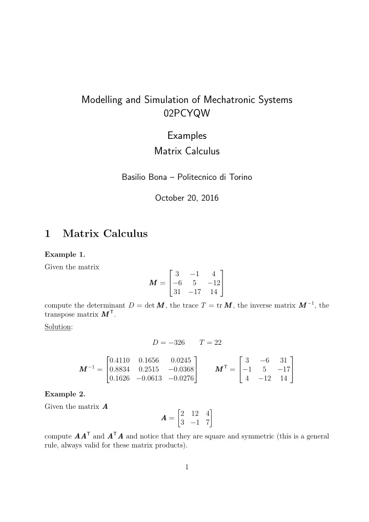
Modelling and Simulation of Mechatronic Systems 02PCYQW Examples Matrix Calculus Basilio Bona – Politecnico di Torino October 20, 2016 1 Matrix Calculus Example 1. Given the matrix   3 − 1 4 M = − 6 5 − 12   31 − 17 14 compute the determinant D = det M , the trace T = tr M , the inverse matrix M − 1 , the transpose matrix M T . Solution: D = − 326 T = 22     0 . 4110 0 . 1656 0 . 0245 3 − 6 31 M − 1 = M T = 0 . 8834 0 . 2515 − 0 . 0368 − 1 5 − 17     0 . 1626 − 0 . 0613 − 0 . 0276 4 − 12 14 Example 2. Given the matrix A � 2 � 12 4 A = 3 − 1 7 compute AA T and A T A and notice that they are square and symmetric (this is a general rule, always valid for these matrix products). 1

Solution:   13 21 29 � 164 � 22 AA T = A T A = 21 145 41   22 59 29 41 65 The rank of AA T is equal to 2, and also the rank of A T A is equal to 2, i.e., the rank of both product matrices in not larger than the rank of the original A . Example 3. Given the square matrix M of Example 1, compute its decomposition M = M s + M ss and the vector v associated to the skew-symmetric matrix M ss Solution:   3 . 0 − 3 . 5 17 . 5 M s = 1 2( M + M T ) = − 3 . 5 5 . 0 − 14 . 5   17 . 5 14 . 5 14 . 0   0 2 . 5 − 13 . 5 M ss = 1 2( M − M T ) = − 2 . 5 0 2 . 5   13 . 5 − 2 . 5 0   − 2 . 5 v = − 13 . 5   − 2 . 5 Example 4. Given the following two matrices A and B     0 . 3473 − 0 . 6016 − 0 . 7193 0 . 3473 0 . 6016 − 0 . 7193 A = 0 . 5702 0 . 7445 − 0 . 3473 B = 0 . 5702 − 0 . 7445 − 0 . 3473     0 . 7445 − 0 . 2895 0 . 6016 0 . 7445 0 . 2895 0 . 6016 find which one is a rotation matrix and which one is a reflection matrix. Solution: Both products A T A and BB T give an identity matrix, so it is necessary to compute the determinant, det( A ) = 1 , while det( B ) = − 1 so B is the reflection matrix. Now, if one performs two successive reflections, that corre- spond to the product BB = B 2 , the resulting matrix has determinant equal to 1, that is, a rotation. 2

Example 5. Recalling the identity that defines a skew-symmetric matrix S S 2 ( v ) = vv T − � v � 2 I use the vector of Example ?? to generate the matrix S and confirm that the vector em- bedded in S is indeed v . Solution:       1 2 3 1 0 0 − 13 2 3 vv T − � v � 2 I =  − 14  = 2 4 6 0 1 0 2 − 10 6     3 6 9 0 0 1 3 6 − 5 Since the generic second power of a skew-symmetric matrix is − ( Z 2 + Y 2 )       0 − Z 0 − Z Y Y XY XZ − ( Z 2 + X 2 )  = 0 − X 0 − X Z Z XY Y Z      − ( Y 2 + X 2 ) − Y 0 − Y 0 X X XZ Y Z one can see that   X = 1 v = Y = 2   Z = 3 satisfies the relation. Example 6. Given two skew-symmetric matrices S 1 , S 2     0 0 2 0 − 1 2 S 1 ( v ) = 0 0 − 1 S 2 ( w ) = 1 0 0     − 2 − 1 0 − 2 0 0 compute the commutator matrix S comm = [ S 1 , S 2 ] Solution: Since [ S 1 , S 2 ] = S 1 S 2 − S 2 S 1 one obtains       − 4 0 0 − 4 2 1 0 − 2 − 1  −  = S comm ( z ) = [ S 1 , S 2 ] = 2 0 0 0 0 2 2 0 − 2     1 2 − 4 0 0 − 4 1 2 0 3

with   2 z = − 1   2 4