Modeling of two-phase flow > Direct steam generation in solar - - PowerPoint PPT Presentation

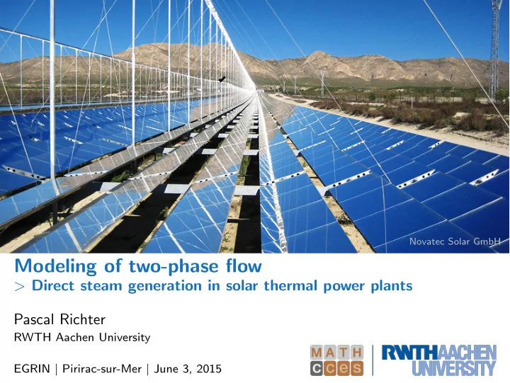
Novatec Solar GmbH

Modeling of two-phase flow

> Direct steam generation in solar thermal power plants Pascal Richter

RWTH Aachen University EGRIN | Pirirac-sur-Mer | June 3, 2015

Direct steam generation | Solar thermal power plant

Solar collector Steam turbine Generator Cooling tower Conden- sator Pump Deaerator Pump

Pascal Richter | Modeling of two-phase flow | 2/14

Direct steam generation | Fresnel collector

Solar collector Steam turbine Generator Cooling tower Conden- sator Pump Deaerator Pump

S u n l i g h t Fresnel Solar collector

• Absorber tube

(two-phase flow)

• Secondary reflector
• Pascal Richter | Modeling of two-phase flow

| 2/14

Direct steam generation | Two-phase flow

Solar collector Steam turbine Generator Cooling tower Conden- sator Pump Deaerator Pump

• Liquid and steam phase in absorber tubes
• Exchange of mass, momentum and energy across the phases
• Interaction of the phases at the wall
• Network coupling

Pascal Richter | Modeling of two-phase flow | 2/14

How to model two-phase flow?

Fluid k, that occupies the observed domain, is described with Navier-Stokes equations: Continuity, momentum and total energy Plenty of models in the literature!

Pascal Richter | Modeling of two-phase flow | 3/14

How to model two-phase flow?

Model development

• Dimension reduction
• Averaging of the Navier-Stokes equations
• Source terms
• Quantities

Density Velocity Energy Pressure 9 > > = > > ; separate, mixture or equal

Pascal Richter | Modeling of two-phase flow | 3/14

How to model two-phase flow?

Model development

• Dimension reduction

! Quasi-1D flow in a tube, Stewart and Wendroff [1]

• Averaging of the Navier-Stokes equations
• Source terms
• Quantities

Density Velocity Energy Pressure 9 > > = > > ; separate, mixture or equal

Pascal Richter | Modeling of two-phase flow | 3/14

How to model two-phase flow?

Model development

• Dimension reduction

! Quasi-1D flow in a tube, Stewart and Wendroff [1]

• Averaging of the Navier-Stokes equations

! Introduction of void fractions α Drew and Passman [2] ! Baer-Nunziato type [3]

• Source terms
• Quantities

Density Velocity Energy Pressure 9 > > = > > ; separate, mixture or equal

Pascal Richter | Modeling of two-phase flow | 3/14

How to model two-phase flow?

Model development

• Dimension reduction

! Quasi-1D flow in a tube, Stewart and Wendroff [1]

• Averaging of the Navier-Stokes equations

! Introduction of void fractions α Drew and Passman [2] ! Baer-Nunziato type [3]

• Source terms: Replace viscous and diffusive terms, RELAP [4]

! Use empirical laws dependent on local flow pattern

• Quantities

Density Velocity Energy Pressure 9 > > = > > ; separate, mixture or equal

Pascal Richter | Modeling of two-phase flow | 3/14

How to model two-phase flow?

Model development

• Dimension reduction

! Quasi-1D flow in a tube, Stewart and Wendroff [1]

• Averaging of the Navier-Stokes equations

! Introduction of void fractions α Drew and Passman [2] ! Baer-Nunziato type [3]

• Source terms: Replace viscous and diffusive terms, RELAP [4]

! Use empirical laws dependent on local flow pattern

• Quantities

Density Velocity Energy Pressure 9 > > = > > ; separate, mixture or equal

Pascal Richter | Modeling of two-phase flow | 3/14

Two-phase flow model

The system is in non-conservative form ∂tu + ∂xf(u) + B(u) ∂xu = s(u), u = B B B B B B B B @ αg α`ρ` α`ρ`v` α`ρ`E` αgρg αgρgvg αgρgEg 1 C C C C C C C C A , f(u) = B B B B B B B B @ α`ρ`v` α`(ρ`v 2

` + p`)

α`(ρ`E` + p`)v` αgρgvg αg(ρgv 2

g + pg)

αg(ρgEg + pg)vg 1 C C C C C C C C A B(u) = B B B B B B B B @ vi pi pivi pi pivi 1 C C C C C C C C A , s(u) = B B B B B B B B @ Γi/ρi Γi Fi viΓi v`Fi + Qi ` Ei `Γi Γi Fi + viΓi vgFi + Qi g + Ei gΓi 1 C C C C C C C C A

Pascal Richter | Modeling of two-phase flow | 4/14

Two-phase flow model

The system is in non-conservative form ∂tu + ∂xf(u) + B(u) ∂xu = s(u), u = B B B B B B B B @ αg α`ρ` α`ρ`v` α`ρ`E` αgρg αgρgvg αgρgEg 1 C C C C C C C C A , f(u) = B B B B B B B B @ α`ρ`v` α`(ρ`v 2

` + p`)

α`(ρ`E` + p`)v` αgρgvg αg(ρgv 2

g + pg)

αg(ρgEg + pg)vg 1 C C C C C C C C A B(u) = B B B B B B B B @ vi pi pivi pi pivi 1 C C C C C C C C A , s(u) = B B B B B B B B @ Γi/ρi Γi Fi viΓi v`Fi + Qi ` Ei `Γi Γi Fi + viΓi vgFi + Qi g + Ei gΓi 1 C C C C C C C C A Model properties

1 Source terms and interphase

quantities

2 Conservation of mass, momentum

and energy at the interface

3 Equation of state

! How to describe pressure p ?

4 Well-posedness of the model

! Hyperbolicity

5 Entropy inequality

! Consistent with 2nd law of thermodynamics

Pascal Richter | Modeling of two-phase flow | 4/14

Two-phase flow model |

1 Source terms B(u) = B B B B B B B B @ vi pi pivi pi pivi 1 C C C C C C C C A , s(u) = B B B B B B B B @ Γi/ρi Γi Fi viΓi v`Fi + Qi ` Ei `Γi Γi Fi + viΓi vgFi + Qi g + Ei gΓi 1 C C C C C C C C A

• Interphase quantities:

Γi, vi, pi, Ei `, Ei g, ρi = ???

• Flow regimes for friction Fi:
• Models for heat transfer Qi `, Qi g:

Convection, Condensation, Nucleate & Film boiling

Pascal Richter | Modeling of two-phase flow | 5/14

Two-phase flow model |

2 Conservation at interface s(u) = B B B B B B B B @ Γi/ρi Γi Fi viΓi v`Fi + Qi ` Ei `Γi Γi Fi + viΓi vgFi + Qi g + Ei gΓi 1 C C C C C C C C A Heat conduction limited model Γi = 1 Ei ` Ei g ⇣ Fi(vg v`) + Qi ` + Qi g ⌘ RELAP [4].

Pascal Richter | Modeling of two-phase flow | 6/14

Two-phase flow model |

3 Equation of state f(u) = B B B B B B B B @ α`ρ`v` α`(ρ`v 2

` + p`)

α`(ρ`E` + p`)v` αgρgvg αg(ρgv 2

g + pg)

αg(ρgEg + pg)vg 1 C C C C C C C C A Describe p by two state parameter p` = p(ρ`, u`), pg = p(ρg, ug) with density ρ and specific inner energy u.

Pascal Richter | Modeling of two-phase flow | 7/14

Two-phase flow model |

4 Hyperbolicity Rewrite system in terms of primitive quantities ∂tw + M(w)∂xw = ˜ s(w) Eigenvalues λ = vi, v`, v` + w`, v` w`, vg, vg + wg, vg wg T with speed of sound w.

Pascal Richter | Modeling of two-phase flow | 8/14

Two-phase flow model |

4 Hyperbolicity Rewrite system in terms of primitive quantities ∂tw + M(w)∂xw = ˜ s(w) Eigenvalues λ = vi, v`, v` + w`, v` w`, vg, vg + wg, vg wg T with speed of sound w. Eigenvectors form a basis of R7 as soon as the non-resonance condition is fulfilled Coquel, H´ erard, Saleh, and Seguin [5] : vi 6= v` ± w` and vi 6= vg ± wg.

Pascal Richter | Modeling of two-phase flow | 8/14

Two-phase flow model |

4 Hyperbolicity Rewrite system in terms of primitive quantities ∂tw + M(w)∂xw = ˜ s(w) Eigenvalues λ = vi, v`, v` + w`, v` w`, vg, vg + wg, vg wg T with speed of sound w. Eigenvectors form a basis of R7 as soon as the non-resonance condition is fulfilled Coquel, H´ erard, Saleh, and Seguin [5] : vi 6= v` ± w` and vi 6= vg ± wg. Gallou¨ et, H´ erard, and Seguin [6] choose vi as convex combination between v` and vg: vi := βv` + (1 β)vg with β 2 [0, 1] Non-resonance condition will always be fulfilled ! M is diagonalisable ! quasilinear system is hyperbolic.

Pascal Richter | Modeling of two-phase flow | 8/14

Two-phase flow model |

5 Entropy-entropy flux pair Closed quasilinear form: ∂tu + A(u) · ∂xu = s(u). Find entropy function η(u) and entropy flux ψ(u), such that ∂tη(u) + ∂xψ(u)

!

 0

Pascal Richter | Modeling of two-phase flow | 9/14

Two-phase flow model |

5 Entropy-entropy flux pair Closed quasilinear form: ∂tu + A(u) · ∂xu = s(u). Find entropy function η(u) and entropy flux ψ(u), such that ∂tη(u) + ∂xψ(u)

!

 0 with

1 Convex entropy (decreasing behaviour):

η00(u) > 0

2 Compatibility condition of Tadmor [8]:

∂uψ(u)T

!

= ∂uη(u)T A(u)

Pascal Richter | Modeling of two-phase flow | 9/14

Two-phase flow model |

5 Entropy-entropy flux pair Closed quasilinear form: ∂tu + A(u) · ∂xu = s(u). Find entropy function η(u) and entropy flux ψ(u), such that ∂tη(u) + ∂xψ(u)

!

 0 with

1 Convex entropy (decreasing behaviour):

η00(u) > 0

2 Compatibility condition of Tadmor [8]:

∂uψ(u)T

!

= ∂uη(u)T A(u)

3 Entropy production condition:

∂tu + A(u) · ∂xu = s(u) , ∂uη(u)T ∂tu + ∂uη(u)T A(u) · ∂xu = ∂uη(u)T s(u) , ∂tη(u) + ∂xψ(u) = ∂uη(u)T s(u)

!

 0

Pascal Richter | Modeling of two-phase flow | 9/14

Two-phase flow model |

5 Entropy-entropy flux pair (1) Choose mixture of physical entropy s` and sg: η(u) = (α`ρ`s` + αgρgsg) and ψ(u) = (α`ρ`s`v` + αgρgsgvg)

Pascal Richter | Modeling of two-phase flow | 10/14

Two-phase flow model |

5 Entropy-entropy flux pair (1) Choose mixture of physical entropy s` and sg: η(u) = (α`ρ`s` + αgρgsg) and ψ(u) = (α`ρ`s`v` + αgρgsgvg)

1 Convexity of η(u):

Follow proof of Coquel, H´ erard, Saleh, and Seguin [5], using results of Godlewski and Raviart [7].

Pascal Richter | Modeling of two-phase flow | 10/14

Two-phase flow model |

5 Entropy-entropy flux pair (2) Choose mixture of physical entropy s` and sg: η(u) = (α`ρ`s` + αgρgsg) and ψ(u) = (α`ρ`s`v` + αgρgsgvg)

2 Compatibility condition

∂uψ(u)T

!

= ∂uη(u)T · A(u):

                      

p`v` T` pgvg Tg

v` ·

p` ⇢` +u` 1 2 v2 ` T` v2 ` T` s`

• v`

T`

vg ·

pg ⇢g +ug 1 2 v2 g Tg v2 g Tg sg

• vg

Tg

                      

!

=                       

p`v` T` pgvg Tg (p`pi)(v`vi) T`

+ (pgpi)(vgvi)

Tg

v` ·

p` ⇢` +u` 1 2 v2 ` T` v2 ` T` s`

• v`

T`

vg ·

pg ⇢g +ug 1 2 v2 g Tg v2 g Tg sg

• vg

Tg

                      

Pascal Richter | Modeling of two-phase flow | 11/14

Two-phase flow model |

5 Entropy-entropy flux pair (2) Choose mixture of physical entropy s` and sg: η(u) = (α`ρ`s` + αgρgsg) and ψ(u) = (α`ρ`s`v` + αgρgsgvg)

2 Compatibility condition

∂uψ(u)T

!

= ∂uη(u)T · A(u):

                      

p`v` T` pgvg Tg

v` ·

p` ⇢` +u` 1 2 v2 ` T` v2 ` T` s`

• v`

T`

vg ·

pg ⇢g +ug 1 2 v2 g Tg v2 g Tg sg

• vg

Tg

                      

!

=                       

p`v` T` pgvg Tg (p`pi)(v`vi) T`

+ (pgpi)(vgvi)

Tg

v` ·

p` ⇢` +u` 1 2 v2 ` T` v2 ` T` s`

• v`

T`

vg ·

pg ⇢g +ug 1 2 v2 g Tg v2 g Tg sg

• vg

Tg

                      

Interphasic velocity [Hyperbolicity] vi = βv` + (1 β)vg with β 2 [0, 1] Interphasic pressure Gallou¨ et, H´ erard, and Seguin [6] pi := γp` + (1 γ)pg with γ 2 [0, 1]

Pascal Richter | Modeling of two-phase flow | 11/14

Two-phase flow model |

5 Entropy-entropy flux pair (2) Choose mixture of physical entropy s` and sg: η(u) = (α`ρ`s` + αgρgsg) and ψ(u) = (α`ρ`s`v` + αgρgsgvg)

2 Compatibility condition

∂uψ(u)T

!

= ∂uη(u)T · A(u):

                      

p`v` T` pgvg Tg

v` ·

p` ⇢` +u` 1 2 v2 ` T` v2 ` T` s`

• v`

T`

vg ·

pg ⇢g +ug 1 2 v2 g Tg v2 g Tg sg

• vg

Tg

                      

!

=                       

p`v` T` pgvg Tg (p`pi)(v`vi) T`

+ (pgpi)(vgvi)

Tg

v` ·

p` ⇢` +u` 1 2 v2 ` T` v2 ` T` s`

• v`

T`

vg ·

pg ⇢g +ug 1 2 v2 g Tg v2 g Tg sg

• vg

Tg

                      

Interphasic velocity [Hyperbolicity] vi = βv` + (1 β)vg with β 2 [0, 1] Interphasic pressure pi := γp` + (1 γ)pg ) γ =

(1)Tg T`+(1)Tg

Pascal Richter | Modeling of two-phase flow | 11/14

Two-phase flow model |

5 Entropy-entropy flux pair (3) Choose mixture of physical entropy s` and sg: η(u) = (α`ρ`s` + αgρgsg) and ψ(u) = (α`ρ`s`v` + αgρgsgvg)

3 Entropy inequality of entropy production:

∂uη(u)T s(u)

!

 0:

− Qi ` T` + Ei ` − E` + v 2

` − v`vi + p` ⇢i − p` ⇢` + s`T`

T` · Γi − Qi g Tg − Ei g − Eg + v 2

g − vgvi + pg ⇢i − pg ⇢g + sgTg

Tg · Γi

!

≤

Pascal Richter | Modeling of two-phase flow | 12/14

Two-phase flow model |

5 Entropy-entropy flux pair (3) Choose mixture of physical entropy s` and sg: η(u) = (α`ρ`s` + αgρgsg) and ψ(u) = (α`ρ`s`v` + αgρgsgvg)

3 Entropy inequality of entropy production:

∂uη(u)T s(u)

!

 0:

− Qi ` T` + Ei ` − E` + v 2

` − v`vi + p` ⇢i − p` ⇢` + s`T`

T` · Γi − Qi g Tg − Ei g − Eg + v 2

g − vgvi + pg ⇢i − pg ⇢g + sgTg

Tg · Γi

!

≤

• Spec. total energy = spec. enthalpy spec. pressure + kinetic energy

(physical law)

E` = h` p`

⇢` + 1 2v 2 ` ,

Ei ` := h` sat pi

⇢i + 1 2v 2 i

Eg = hg pg

⇢g + 1 2v 2 g ,

Ei g := hg sat pi

⇢i + 1 2v 2 i

Pascal Richter | Modeling of two-phase flow | 12/14

Two-phase flow model |

5 Entropy-entropy flux pair (3) Choose mixture of physical entropy s` and sg: η(u) = (α`ρ`s` + αgρgsg) and ψ(u) = (α`ρ`s`v` + αgρgsgvg)

3 Entropy inequality of entropy production:

∂uη(u)T s(u)

!

 0:

− Qi ` T` + h` sat − h` + 1

2(v` − vi)2 + p`pi ⇢i

+ s`T` T` · Γi − Qi g Tg − hg sat − hg + 1

2(vg − vi)2 + pg pi ⇢i

+ sgTg Tg · Γi

!

≤

• Spec. total energy = spec. enthalpy spec. pressure + kinetic energy

(physical law)

E` = h` p`

⇢` + 1 2v 2 ` ,

Ei ` := h` sat pi

⇢i + 1 2v 2 i

Eg = hg pg

⇢g + 1 2v 2 g ,

Ei g := hg sat pi

⇢i + 1 2v 2 i

Pascal Richter | Modeling of two-phase flow | 12/14

Two-phase flow model |

5 Entropy-entropy flux pair (3) Choose mixture of physical entropy s` and sg: η(u) = (α`ρ`s` + αgρgsg) and ψ(u) = (α`ρ`s`v` + αgρgsgvg)

3 Entropy inequality of entropy production:

∂uη(u)T s(u)

!

 0:

− Qi ` T` + h` sat − h` + 1

2(v` − vi)2 + p`pi ⇢i

+ s`T` T` · Γi − Qi g Tg − hg sat − hg + 1

2(vg − vi)2 + pg pi ⇢i

+ sgTg Tg · Γi

!

≤

• Spec. total energy = spec. enthalpy spec. pressure + kinetic energy

(physical law)

E` = h` p`

⇢` + 1 2v 2 ` ,

Ei ` := h` sat pi

⇢i + 1 2v 2 i

Eg = hg pg

⇢g + 1 2v 2 g ,

Ei g := hg sat pi

⇢i + 1 2v 2 i

Interphasic velocity vi := βv` + (1 β)vg with β 2 [0, 1]

Pascal Richter | Modeling of two-phase flow | 12/14

Two-phase flow model |

5 Entropy-entropy flux pair (3) Choose mixture of physical entropy s` and sg: η(u) = (α`ρ`s` + αgρgsg) and ψ(u) = (α`ρ`s`v` + αgρgsgvg)

3 Entropy inequality of entropy production:

∂uη(u)T s(u)

!

 0:

− Qi ` T` + h` sat − h` + 1

2(v` − vi)2 + p`pi ⇢i

+ s`T` T` · Γi − Qi g Tg − hg sat − hg + 1

2(vg − vi)2 + pg pi ⇢i

+ sgTg Tg · Γi

!

≤

• Spec. total energy = spec. enthalpy spec. pressure + kinetic energy

(physical law)

E` = h` p`

⇢` + 1 2v 2 ` ,

Ei ` := h` sat pi

⇢i + 1 2v 2 i

Eg = hg pg

⇢g + 1 2v 2 g ,

Ei g := hg sat pi

⇢i + 1 2v 2 i

Interphasic velocity vi := βv` + (1 β)vg ) β :=

√

Tg pT`+√ Tg

Pascal Richter | Modeling of two-phase flow | 12/14

Two-phase flow model |

5 Entropy-entropy flux pair (3) Choose mixture of physical entropy s` and sg: η(u) = (α`ρ`s` + αgρgsg) and ψ(u) = (α`ρ`s`v` + αgρgsgvg)

3 Entropy inequality of entropy production:

∂uη(u)T s(u)

!

 0:

− Qi ` T` + h` sat − h` + p`pi

⇢i

+ s`T` T` · Γi − Qi g Tg − hg sat − hg + pg pi

⇢i

+ sgTg Tg · Γi

!

≤

• Spec. total energy = spec. enthalpy spec. pressure + kinetic energy

(physical law)

E` = h` p`

⇢` + 1 2v 2 ` ,

Ei ` := h` sat pi

⇢i + 1 2v 2 i

Eg = hg pg

⇢g + 1 2v 2 g ,

Ei g := hg sat pi

⇢i + 1 2v 2 i

Interphasic velocity vi := βv` + (1 β)vg ) β :=

√

Tg pT`+√ Tg

Pascal Richter | Modeling of two-phase flow | 12/14

Two-phase flow model |

5 Entropy-entropy flux pair (3) Choose mixture of physical entropy s` and sg: η(u) = (α`ρ`s` + αgρgsg) and ψ(u) = (α`ρ`s`v` + αgρgsgvg)

3 Entropy inequality of entropy production:

∂uη(u)T s(u)

!

 0:

− Qi ` T` + h` sat − h` + p`pi

⇢i

+ s`T` T` · Γi − Qi g Tg − hg sat − hg + pg pi

⇢i

+ sgTg Tg · Γi

!

≤

• Spec. total energy = spec. enthalpy spec. pressure + kinetic energy

(physical law)

E` = h` p`

⇢` + 1 2v 2 ` ,

Ei ` := h` sat pi

⇢i + 1 2v 2 i

Eg = hg pg

⇢g + 1 2v 2 g ,

Ei g := hg sat pi

⇢i + 1 2v 2 i

Interphasic velocity vi := βv` + (1 β)vg ) β :=

√

Tg pT`+√ Tg

Interphasic density ρi := ρsat

Pascal Richter | Modeling of two-phase flow | 12/14

Two-phase flow model |

5 Entropy-entropy flux pair (3) Choose mixture of physical entropy s` and sg: η(u) = (α`ρ`s` + αgρgsg) and ψ(u) = (α`ρ`s`v` + αgρgsgvg)

3 Entropy inequality of entropy production:

∂uη(u)T s(u)

!

 0:

− Qi ` T` + h` sat − h` + p`pi

⇢i

+ s`T` T` · Γi − Qi g Tg − hg sat − hg + pg pi

⇢i

+ sgTg Tg · Γi

!

≤

• Spec. total energy = spec. enthalpy spec. pressure + kinetic energy

(physical law)

E` = h` p`

⇢` + 1 2v 2 ` ,

Ei ` := h` sat pi

⇢i + 1 2v 2 i

Eg = hg pg

⇢g + 1 2v 2 g ,

Ei g := hg sat pi

⇢i + 1 2v 2 i

Interphasic velocity vi := βv` + (1 β)vg ) β :=

√

Tg pT`+√ Tg

Interphasic density ρi := ρsat ! Check entropy inequality within physical relevant region!

Pascal Richter | Modeling of two-phase flow | 12/14

Two-phase flow model | Summary

Model properties X Source terms and interphase quantities X Conservation of mass, momentum and energy at the interface X Equation of state X Well-posed hyperbolic model X Entropy-Entropy flux pair Consistent with 2nd law of thermodynamics

Pascal Richter | Modeling of two-phase flow | 13/14

Two-phase flow model | Summary

Model properties X Source terms and interphase quantities X Conservation of mass, momentum and energy at the interface X Equation of state X Well-posed hyperbolic model X Entropy-Entropy flux pair Consistent with 2nd law of thermodynamics No linear degenerated field for first eigenvalue λ1 = vi,

• nly iff vi := v`,
• r

vi := vg,

• r

vi := ↵`⇢`v`+↵g⇢gvg

↵`⇢`+↵g⇢g

.

Pascal Richter | Modeling of two-phase flow | 13/14

Two-phase flow model | Next steps

Numerical schemes for quasilinear system

1 Path-conservative scheme, Castro et al. [10]

• transform into homogeneous system in non-conservative form
• path connects two states uL and uR at its left xL and right xR limits

across a discontinuity

2 Relaxation, Baudin, Berthon, Coquel, Masson, and Tran [11]

• transform system, such that it is linearly degenerated (?)
• extend system with relaxed pressure and temperature equations
• system linearly degenerate → easy to find Riemann solution.

Pascal Richter | Modeling of two-phase flow | 14/14

Bibliography I

H.B. Stewart and B. Wendroff. “Two-phase flow: models and methods” . In: Journal of Computational Physics 56.3 (1984), pp. 363–409. D.A. Drew and S.L. Passman. Theory of Multicomponent Fluids. Applied mathematical

• sciences. Springer, 1998.

M.R. Baer and J.W. Nunziato. “A two-phase mixture theory for the deflagration-to-detonation transition (DDT) in reactive granular materials” . In: International Journal of Multiphase Flow 12.6 (1986), pp. 861–889. Idaho National Laboratory. RELAP5-3D c

Code Manual Volume I: Code Structure,

System Models and Solution Methods. Tech. rep. INL Idaho National Laboratory (INL), INEEL Report EXT-98-00834, Revision 4.0, 2012.

• F. Coquel et al. “Two properties of two-velocity two-pressure models for two-phase flows”

. In: (2013).

• T. Gallou¨

et, J.-M. H´ erard, and N. Seguin. “Numerical modeling of two-phase flows using the two-fluid two-pressure approach” . In: Mathematical Models and Methods in Applied Sciences 14.05 (2004), pp. 663–700.

Pascal Richter | Modeling of two-phase flow | 13/14

Bibliography II

• E. Godlewski and P.-A. Raviart. Numerical approximation of hyperbolic systems of

conservation laws. Vol. 118. Springer, 1996.

• E. Tadmor. “The numerical viscosity of entropy stable schemes for systems of conservation
• laws. I”

. In: Mathematics of Computation 49.179 (1987), pp. 91–103. A Zein. “Numerical methods for multiphase mixture conservation laws with phase transition” . PhD thesis. University of Magdeburg, 2010. M.J. Castro et al. “Entropy Conservative and Entropy Stable Schemes for Nonconservative Hyperbolic Systems” . In: SIAM Journal on Numerical Analysis 51.3 (2013), pp. 1371–1391. Micha¨ el Baudin et al. “A relaxation method for two-phase flow models with hydrodynamic closure law” . In: Numerische Mathematik 99.3 (2005), pp. 411–440.

Pascal Richter | Modeling of two-phase flow | 14/14