Mixed models in R using the lme4 package Part 3: Inference based on - PDF document

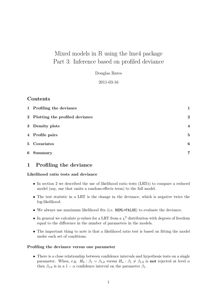
Mixed models in R using the lme4 package Part 3: Inference based on profiled deviance Douglas Bates 2011-03-16 Contents 1 Profiling the deviance 1 2 Plotting the profiled deviance 2 3 Density plots 4 4 Profile pairs 5 5 Covariates 6 6 Summary 7 1 Profiling the deviance Likelihood ratio tests and deviance • In section 2 we described the use of likelihood ratio tests (LRTs) to compare a reduced model (say, one that omits a random-effects term) to the full model. • The test statistic in a LRT is the change in the deviance, which is negative twice the log-likelihood. • We always use maximum likelihood fits (i.e. REML=FALSE ) to evaluate the deviance. • In general we calculate p-values for a LRT from a χ 2 distribution with degrees of freedom equal to the difference in the number of parameters in the models. • The important thing to note is that a likelihood ratio test is based on fitting the model under each set of conditions. Profiling the deviance versus one parameter • There is a close relationship between confidence intervals and hypothesis tests on a single parameter. When, e.g. H 0 : β 1 = β 1 , 0 versus H a : β 1 � = β 1 , 0 is not rejected at level α then β 1 , 0 is in a 1 − α confidence interval on the parameter β 1 . 1

log ( σ ) σ 1 (Intercept) 2 1 ζ 0 −1 −2 0 20 40 60 80 100 3.6 3.8 4.0 4.2 1500 1550 Figure 1: Profile plot of the parameters in model fm1M • For linear fixed-effects models it is possible to determine the change in the deviance from fitting the full model only. For mixed-effects models we need to fit the full model and all the reduced models to perform the LRTs. • In practice we fit some of them and use interpolation. The profile function evaluates such a “profile” of the change in the deviance versus each of the parameters in the model. Transforming the LRT statistic • The LRT statistic for a test of a fixed value of a single parameter would have a χ 2 1 distribution, which is the square of a standard normal. • If a symmetric confidence interval were appropriate for the parameter, the LRT statistic would be quadratic with respect to the parameter. • We plot the square root of the LRT statistic because it is easier to assess whether the plot looks like a straight line than it is to assess if it looks like a quadratic. • To accentuate the straight line behavior we use the signed square root transformation which returns the negative square root to the left of the estimate and the positive square root to the right. • This quantity can be compared to a standard normal. We write it as ζ 2 Plotting the profiled deviance Evaluating and plotting the profile Figure 1 is produced as > pr1 <- profile(fm1M <- lmer(Yield ~ 1+(1| Batch), Dyestuff , REML=FALSE )) > xyplot(pr1 , aspect =1.3) • The parameters are σ b , log( σ ) ( σ is the residual standard deviation) and µ . The vertical lines delimit 50%, 80%, 90%, 95% and 99% confidence intervals. Figure 2 is produced as 2

2.5 2.0 (Intercept) log ( σ ) 1.5 | ζ | σ 1 1.0 0.5 0.0 0 20 40 60 80 100 3.6 3.8 4.0 4.2 1500 1550 Figure 2: Alternative profile plot using absVal=TRUE for the parameters in model lm1 > xyplot(pr1 , aspect =0.7, absVal=TRUE) Numerical values of the confidence interval limits are obtained from the method for the confint generic > confint(pr1) 2.5 % 97.5 % .sig01 12.201753 84.06289 .lsig 3.643622 4.21446 (Intercept) 1486.451500 1568.54849 Changing the confidence level As for other methods for the confint generic, we use level= α to obtain a confidence level other than the default of 0 . 95. > confint(pr1 , level =0.99) 0.5 % 99.5 % .sig01 NA 113.692643 .lsig 3.571293 4.326347 (Intercept) 1465.874011 1589.126022 Note that the lower 99% confidence limit for σ 1 is undefined. Interpreting the univariate plots • A univariate profile ζ plot is read like a normal probability plot – a sigmoidal (elongated“S”-shaped) pattern like that for the (Intercept) parameter indicates overdispersion relative to the normal distribution. – a bending pattern, usually flattening to the right of the estimate, indicates skewness of the estimator and warns us that the confidence intervals will be asymmetric – a straight line indicates that the confidence intervals based on the quantiles of the standard normal distribution are suitable • Note that the only parameter providing a more-or-less straight line is σ and this plot is on the scale of log( σ ) not σ or, even worse, σ 2 . 3

log ( σ ) σ σ 2 2 1 ζ 0 −1 −2 3.6 3.8 4.0 4.2 40 50 60 70 2000 3000 4000 5000 Figure 3: Profile ζ plots for log( σ ), σ and σ 2 in model fm1ML log ( σ 1 ) σ 1 σ 1 2 2 1 0 ζ −1 −2 2 3 4 0 20 40 60 80 100 0 5000 10000 Figure 4: Profile ζ plots for log( σ 1 ), σ 1 and σ 2 1 in model fm1ML • We should expect confidence intervals on σ 2 to be asymmetric. In the simplest case of a variance estimate from an i.i.d. normal sample the confidence interval is derived from quantiles of a χ 2 distribution which is quite asymmetric (although many software packages provide standard errors of variance component estimates as if they were mean- ingful). In Fig. 3 • We can see moderate asymmetry on the scale of σ and stronger asymmetry on the scale of σ 2 . • The issue of which of the ML or REML estimates of σ 2 are closer to being unbiased is a red herring. σ 2 is not a sensible scale on which to evaluate the expected value of an estimator. In Fig. 4 we see • For σ 1 the situation is more complicated because 0 is within the range of reasonable values. The profile flattens as σ → 0 which means that intervals on log( σ ) are unbounded. • Obviously the estimator of σ 2 1 is terribly skewed yet most software ignores this and provides standard errors on variance component estimates. 4

3 Density plots Converting profile ζ to a density • We speak of a profile ζ plot as showing skewness, especially for parameters such as σ 1 and σ . • Often it is easier to envision symmetry or skewness in terms of a density plot. • If ζ is compared to a standard Gaussian distribution then the corresponding cumulative distribution function is Φ( ζ ), from which we can derive a density function. 0.020 (Intercept) 0.010 0.000 1450 1500 1550 1600 0.0 0.5 1.0 1.5 2.0 2.5 density log ( σ ) 3.6 3.8 4.0 4.2 4.4 0.020 σ 1 0.010 0.000 0 50 100 150 Figure 5: Profile-based densities for the parameters in model fm1 4 Profile pairs Profile pairs plots • The information from the profile can be used to produce pairwise projections of likelihood contours. These correspond to pairwise joint confidence regions. • Such a plot (next slide) can be somewhat confusing at first glance. • Concentrate initially on the panels above the diagonal where the axes are the parameters in the scale shown in the diagonal panels. The contours correspond to 50%, 80%, 90%, 95% and 99% pairwise confidence regions. • The two lines in each panel are “profile traces”, which are the conditional estimate of one parameter given a value of the other. 5

1600 1550 (Intercept) 1500 0 1 2 3 1450 4.4 4.0 4.2 4.4 4.2 4.0 .lsig 3.8 3.6 0 1 2 3 0 50 100 150 .sig01 0 −1 −2 −3 Scatter Plot Matrix Figure 6: Profile pairs for model fm1 • The actual interpolation of the contours is performed on the ζ scale which is shown in the panels below the diagonal. Figure 6 is produced by > splom(pr1) 5 Profiling models with fixed-effects for covariates About those p-values • Statisticians have been far too successful in propagating concepts of hypothesis testing and p-values, to the extent that quoting p-values is essentially a requirement for publi- cation in some disciplines. • When models were being fit by hand calculation it was important to use any trick we could come up with to simplify the calculation. Often the results were presented in terms of the simplified calculation without reference to the original idea of comparing models. • We often still present model comparisons as properties of “terms” in the model without being explicit about the underlying comparison of models with the term and without the term. • The approach I recommend for assessing the importance of particular terms in the fixed- effects part of the model is to fit with and without then use a likelihood ratio test (the anova function). Hypothesis tests versus confidence intervals • As mentioned earlier, hypothesis tests and confidence intervals are two sides of the same coin. 6