
SLIDE 1
Mixed Mimetic Spectral Elements for Atmospheric Simulation
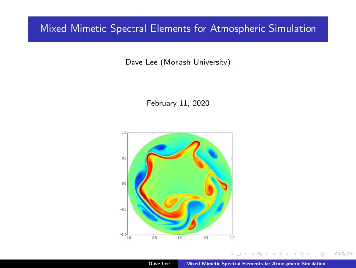
Dave Lee (Monash University) February 11, 2020
Dave Lee Mixed Mimetic Spectral Elements for Atmospheric Simulation
Mixed Mimetic Spectral Elements for Atmospheric Simulation Dave Lee - - PowerPoint PPT Presentation
Mixed Mimetic Spectral Elements for Atmospheric Simulation Dave Lee (Monash University) February 11, 2020 Dave Lee Mixed Mimetic Spectral Elements for Atmospheric Simulation Motivation Improved representation of dynamical processes and long
Dave Lee Mixed Mimetic Spectral Elements for Atmospheric Simulation
∂z = −g
Dave Lee Mixed Mimetic Spectral Elements for Atmospheric Simulation
b b
b b
Dave Lee Mixed Mimetic Spectral Elements for Atmospheric Simulation
ξ
0.5 1 li(ξ)
0.5 1 1.5 2 2.5 3 ξ
0.5 1 ei(ξ)
0.5 1 1.5 2 2.5 3
Dave Lee Mixed Mimetic Spectral Elements for Atmospheric Simulation
Dave Lee Mixed Mimetic Spectral Elements for Atmospheric Simulation
b b
ω2 ψ0
i
p2 φ0,i ψ0 → ∇⊥ → u1 → ∇· → p2 ω2 ← ∇× ← u1 ← ∇ ← φ0 ⋆ ⋆ ⋆
b b
ψ0
i+1
φ0,i+1
Dave Lee Mixed Mimetic Spectral Elements for Atmospheric Simulation
Dave Lee Mixed Mimetic Spectral Elements for Atmospheric Simulation
Dave Lee Mixed Mimetic Spectral Elements for Atmospheric Simulation
Mixed Mimetic Spectral Elements for Atmospheric Simulation
Dave Lee Mixed Mimetic Spectral Elements for Atmospheric Simulation
2 4 6 8 10 10-7 10-6 10-5 Williamson TC2, conservation error, vorticity (un-normalized) ∆x =768km,∆t =150s ∆x =768km,∆t =300s ∆x =384km,∆t =300s 2 4 6 8 10 10-11 10-10 10-9 10-8 10-7 10-6 10-5 Williamson TC2, conservation error, energy ∆x =768km,∆t =150s ∆x =768km,∆t =300s ∆x =384km,∆t =300s 1 2 3 4 5 time (days) 2.0 2.5 3.0 3.5 4.0 4.5 5.0 log2(|L2(∆x)|/|L2(∆x/2)|) Log2 of ratio of L2 errors with doubling of resolution ωh +fh ,(Ne =4)/(Ne =8) ~ uh ,(Ne =4)/(Ne =8) hh ,(Ne =4)/(Ne =8) ωh +fh ,(Ne =8)/(Ne =16) ~ uh ,(Ne =8)/(Ne =16) hh ,(Ne =8)/(Ne =16)
Dave Lee Mixed Mimetic Spectral Elements for Atmospheric Simulation
Dave Lee Mixed Mimetic Spectral Elements for Atmospheric Simulation
Dave Lee Mixed Mimetic Spectral Elements for Atmospheric Simulation
Dave Lee Mixed Mimetic Spectral Elements for Atmospheric Simulation
Dave Lee Mixed Mimetic Spectral Elements for Atmospheric Simulation
Dave Lee Mixed Mimetic Spectral Elements for Atmospheric Simulation
Dave Lee Mixed Mimetic Spectral Elements for Atmospheric Simulation
Dave Lee Mixed Mimetic Spectral Elements for Atmospheric Simulation
Dave Lee Mixed Mimetic Spectral Elements for Atmospheric Simulation
Dave Lee Mixed Mimetic Spectral Elements for Atmospheric Simulation
Dave Lee Mixed Mimetic Spectral Elements for Atmospheric Simulation
Dave Lee Mixed Mimetic Spectral Elements for Atmospheric Simulation