MHD Turbulence Under the Virtual Microscope Gregory L. Eyink - - PowerPoint PPT Presentation

mhd turbulence under the virtual microscope gregory l
SMART_READER_LITE
LIVE PREVIEW

MHD Turbulence Under the Virtual Microscope Gregory L. Eyink - - PowerPoint PPT Presentation

MHD Turbulence Under the Virtual Microscope Gregory L. Eyink Applied Mathematics & Statistics and Physics & Astronomy The Johns Hopkins University 8th International Conference on Numerical Modeling of Space Plasma Flows July 1st -


slide-1
SLIDE 1

MHD Turbulence Under the Virtual Microscope Gregory L. Eyink Applied Mathematics & Statistics and Physics & Astronomy The Johns Hopkins University

8th International Conference on Numerical Modeling of Space Plasma Flows July 1st - July 5th 2013, Biarritz, France Collaborators: JHU Turbulence Database Group (E. Vishniac, C. Meneveau,

  • A. Szalay, R. Burns, H. Aluie, C. Lalescu, K. Kanov) & A. Lazarian
slide-2
SLIDE 2

MHD Turbulence Under the Virtual Microscope Gregory L. Eyink Applied Mathematics & Statistics and Physics & Astronomy The Johns Hopkins University

8th International Conference on Numerical Modeling of Space Plasma Flows July 1st - July 5th 2013, Biarritz, France Collaborators: JHU Turbulence Database Group (E. Vishniac, C. Meneveau,

  • A. Szalay, R. Burns, H. Aluie, C. Lalescu, K. Kanov) & A. Lazarian

This talk will complement yesterday’s by Alex Lazarian!

slide-3
SLIDE 3

MHD Turbulence Under the Virtual Microscope Stochastic Flux-Freezing in MHD Turbulence Gregory L. Eyink Applied Mathematics & Statistics and Physics & Astronomy The Johns Hopkins University

8th International Conference on Numerical Modeling of Space Plasma Flows July 1st - July 5th 2013, Biarritz, France Collaborators: JHU Turbulence Database Group (E. Vishniac, C. Meneveau,

  • A. Szalay, R. Burns, H. Aluie, C. Lalescu, K. Kanov) & A. Lazarian

This talk will complement yesterday’s by Alex Lazarian!

slide-4
SLIDE 4

Representative Calculation (global GR MHD simulation of a thin disk)

The Astrophysical Journal, 769:156 (20pp), 2013 June 1 Schnittman, Krolik, & Noble Figure 2. Fluid density profile for a slice of Harm3d data in the (r, z) plane at simulation time t = 12,500M. Contours show surfaces of constant optical depth with τ = 0.01, 0.1, 1.0. Fiducial values for the black hole mass M = 10 M and accretion rate ˙ m = 0.1 were used. (A color version of this figure is available in the online journal.) Figure 3. Magnetic energy density profile for a slice of Harm3d data in the (r, z) plane corresponding to the same conditions as in Figure 2. (A color version of this figure is available in the online journal.)

“...because an adequate description of MHD turbulence requires a wide dynamic range in length scales (Hawley et al. 2011; Sorathia et al. 2012), the spatial resolution necessary to simulate disks as thin as some of those likely to occur in nature remains beyond our grasp. Thus, in some respects, our calculations represent an intermediate step toward drawing a complete connection between fundamental physics and output spectra.”

  • Schnittman et al. (2013)
slide-5
SLIDE 5

Representative Calculation (global GR MHD simulation of a thin disk)

The Astrophysical Journal, 769:156 (20pp), 2013 June 1 Schnittman, Krolik, & Noble Figure 2. Fluid density profile for a slice of Harm3d data in the (r, z) plane at simulation time t = 12,500M. Contours show surfaces of constant optical depth with τ = 0.01, 0.1, 1.0. Fiducial values for the black hole mass M = 10 M and accretion rate ˙ m = 0.1 were used. (A color version of this figure is available in the online journal.) Figure 3. Magnetic energy density profile for a slice of Harm3d data in the (r, z) plane corresponding to the same conditions as in Figure 2. (A color version of this figure is available in the online journal.)

“...because an adequate description of MHD turbulence requires a wide dynamic range in length scales (Hawley et al. 2011; Sorathia et al. 2012), the spatial resolution necessary to simulate disks as thin as some of those likely to occur in nature remains beyond our grasp. Thus, in some respects, our calculations represent an intermediate step toward drawing a complete connection between fundamental physics and output spectra.”

  • Schnittman et al. (2013)
slide-6
SLIDE 6

turbulence.pha.jhu.edu

Welcome to the JHU Turbulence Database Cluster (TDC) site

This website is a portal that enables access to multi-Terabyte turbulence databases. The data reside on several nodes and disks on our database cluster computer and are stored in small 3D subcubes. Positions are indexed using a Z-curve for efficient access. Access to the data is facilitated by a Web services interface that permits numerical experiments to be run across the Internet. We offer C, Fortran and Matlab interfaces layered above Web services so that scientists can use familiar programming tools on their client platforms. Calls to fetch subsets of the data can be made directly from within a program being executed on the client's platform. Manual queries for data at individual points and times via web-browser are also supported. Evaluation of velocity and pressure at arbitrary points and time is supported using interpolations executed on the database

  • nodes. Spatial differentiation using various order approximations (up to 8th order) are also

supported (for details, see documentation page). Other functions such as spatial filtering are being developed. So far the database contains a 10244 space-time history of a direct numerical simulation (DNS) of isotropic turbulent flow, in incompressible fluid in 3D, and a DNS of the incompressible magneto-hydrodynamic (MHD) equations. The simulations were performed using 1024 grid points in each direction using a pseudo-spectral method, and forcing at large scales. The database allows access to 1024 time steps covering about

  • ne integral turn-over time-scale of the turbulence. The datasets comprise 27 Terabytes

for the isotropic turbulence data and 56 Terabytes for the MHD data. Basic characteristics

  • f the data sets can be found in the datasets description page. Technical details about the

database techniques used for this project are described in the publications. The Turbulence Database Cluster project is funded by the US National Science Foundation . Questions and comments? turbulence@pha.jhu.edu

269903764678 points queried

Please excuse our dust as we continue to develop this site. The Turbulence Database is on-line but may periodcally be unavailable as we continue to add functionalities.

slide-7
SLIDE 7

Figure 6. Snippet of the FORTRAN code running on local user machine. Bold font highlights the lines invoking the Web-services method. The authkey has been intentionally marked out.

slide-8
SLIDE 8

Energy Spectra for JHU MHD Turbulence Database

Figure 1: Spectra of velocity (red) and magnetic (blue) fields

10 10

1

10

2

10

−8

10

−6

10

−4

10

−2

k −3/2 k −5/3 k E u(k), E b(k)

Figure 2: Spectra of Elsasser variables, z+=u+b (red) and z-=u-b (blue)

10 10

1

10

2

10

−8

10

−6

10

−4

10

−2

k −3/2 k −5/3 k E +(k), E −(k)

The spectral exponents are closer to -3/2 than to -5/3, as usual for MHD simulations at these Reynolds numbers (Re ≈ 1170). This fact motivated the Boldyrev theory with α = 1, which gives δu(r⊥) ∼ r1/4

and −3/2 spectrum.

slide-9
SLIDE 9

Energy Spectra for JHU MHD Turbulence Database

Figure 1: Spectra of velocity (red) and magnetic (blue) fields

10 10

1

10

2

10

−8

10

−6

10

−4

10

−2

k −3/2 k −5/3 k E u(k), E b(k)

Figure 2: Spectra of Elsasser variables, z+=u+b (red) and z-=u-b (blue)

10 10

1

10

2

10

−8

10

−6

10

−4

10

−2

k −3/2 k −5/3 k E +(k), E −(k)

The spectral exponents are closer to -3/2 than to -5/3, as usual for MHD simulations at these Reynolds numbers (Re ≈ 1170). This fact motivated the Boldyrev theory with α = 1, which gives δu(r⊥) ∼ r1/4

and −3/2 spectrum. However, see A. Beresnyak, PRL 106 075001 (2011)! The spectral scaling of MHD turbu- lence at astrophysically relevant Reynolds numbers is still being debated....

slide-10
SLIDE 10

Magnetic Flux-Freezing “In view of the infinite conductivity, every motion (perpendicular to the field)

  • f the liquid in relation to the lines of force is forbidden because it would give

infinite eddy currents. Thus the matter of the liquid is ‘fastened’ to the lines

  • f force.” (H. Alfv´

en, 1942) Field-lines do not really move! It is permissible to ascribe a velocity u to the lines of force of magnetic field B if and only if E + 1

cu×B = −∇Φ, or

∂tB = ∇×(u×B). (∗) (W. A. Newcomb, 1958). A flux-preserving velocity u is not usually unique,

  • cf. Newcomb (1958), Vasyliunas (1972), Alfv´

en (1976).

slide-11
SLIDE 11

Magnetic Flux-Freezing “In view of the infinite conductivity, every motion (perpendicular to the field)

  • f the liquid in relation to the lines of force is forbidden because it would give

infinite eddy currents. Thus the matter of the liquid is ‘fastened’ to the lines

  • f force.” (H. Alfv´

en, 1942) Field-lines do not really move! It is permissible to ascribe a velocity u to the lines of force of magnetic field B if and only if E + 1

cu×B = −∇Φ, or

∂tB = ∇×(u×B). (∗) (W. A. Newcomb, 1958). A flux-preserving velocity u is not usually unique,

  • cf. Newcomb (1958), Vasyliunas (1972), Alfv´

en (1976). In fact, even if (*) holds to an extremely good approximation, standard flux- freezing is generally false, under realistic astrophysical conditions!

slide-12
SLIDE 12

Magnetic Flux-Freezing “In view of the infinite conductivity, every motion (perpendicular to the field)

  • f the liquid in relation to the lines of force is forbidden because it would give

infinite eddy currents. Thus the matter of the liquid is ‘fastened’ to the lines

  • f force.” (H. Alfv´

en, 1942) Field-lines do not really move! It is permissible to ascribe a velocity u to the lines of force of magnetic field B if and only if E + 1

cu×B = −∇Φ, or

∂tB = ∇×(u×B). (∗) (W. A. Newcomb, 1958). A flux-preserving velocity u is not usually unique,

  • cf. Newcomb (1958), Vasyliunas (1972), Alfv´

en (1976). In fact, even if (*) holds to an extremely good approximation, standard flux- freezing is generally false, under realistic astrophysical conditions! In turbulent plasmas with power-law spectra of velocity and magnetic fields, flux-freezing does not hold in the standard sense but neither is it completely

  • broken. Instead, flux-freezing becomes intrinsically stochastic.
slide-13
SLIDE 13

Stochastic Flux-Freezing for Resistive MHD The exact solution of the resistive induction equation ∂tB = ∇×(u×B) + λ△B is given by a stochastic Lundquist formula (Eyink 2009, 2011)

B(x, t) =

  • B0(a)·∇a˜

xt,t0(a)

det(∇a˜

xt,t0(a))

  • ˜

xt,t0(a)=x

  • .

Here the average · is over an ensemble of stochastic flows generated by dt˜

xt,t0(a) = u(˜ xt,t0(a), t)dt +

√ 2λ d ˜

W(t),

˜

xt0,t0(a) = a,

where ˜

W(t) is a random Brownian motion.

This is equivalent to a path-integral formula or “sum-over-histories”,

B(x, t) =

  • a(t)=x

Da B0(a(t0))·J(a, t, t0) exp

  • − 1

t

t0

dτ |˙

a(τ) − uν(a(τ), τ)|2

  • where the matrix J satisfies the ODE along the stochastic trajectory a(τ)

d dτ J(a, τ, t0) = J(a, τ, t0)∇xu(a(τ), τ) − J(a, τ, t0)(∇x·u)(a(τ), τ), ,

J(a, t0, t0) = I.

slide-14
SLIDE 14

Stochastic Flux-Freezing for Resistive MHD The exact solution of the resistive induction equation ∂tB = ∇×(u×B) + λ△B is given by a stochastic Lundquist formula (Eyink 2009, 2011)

B(x, t) =

  • B0(a)·∇a˜

xt,t0(a)

det(∇a˜

xt,t0(a))

  • ˜

xt,t0(a)=x

  • .

Here the average · is over an ensemble of stochastic flows generated by dt˜

xt,t0(a) = u(˜ xt,t0(a), t)dt +

√ 2λ d ˜

W(t),

˜

xt0,t0(a) = a,

where ˜

W(t) is a random Brownian motion.

This is equivalent to a path-integral formula or “sum-over-histories”,

B(x, t) =

  • a(t)=x

Da B0(a(t0))·J(a, t, t0) exp

  • − 1

t

t0

dτ |˙

a(τ) − uν(a(τ), τ)|2

  • where the matrix J satisfies the ODE along the stochastic trajectory a(τ)

d dτ J(a, τ, t0) = J(a, τ, t0)∇xu(a(τ), τ) − J(a, τ, t0)(∇x·u)(a(τ), τ), ,

J(a, t0, t0) = I.

We shall see that magnetic field evolution in the presence of fluid turbulence becomes as indeterministic as quantum mechanics and requires similar methods for its description!

slide-15
SLIDE 15

Stochastic Lundquist Formula

B(x, t) =

  • B(a, t0)·∇a˜

xt,t0(a)

det(∇a˜

xt,t0(a))

  • ˜

xt,t0(a)=x

  • 3.12

3.13 3.16

transport

(d/dτ)˜

B = ˜ B·∇u − (∇·u)˜ B

start

x(τ) = u(˜ x, τ)dτ +

√ 2λ d ˜

W(τ)

average

B(x, t) = ˜ B(x, t)

slide-16
SLIDE 16

The Standard View of Flux-Freezing at High Conductivity

It is not hard to show for a smooth velocity field u satisfying |u(x, t) − u(x′, t)| ≤ K|x − x′| that

xt,t0(a) − xt,t0(a)|2

≤ 3λe2Kt − 1 K . = 6λt for Kt ≪ 1. Here xt,t0(a) is the deterministic flow that solves d dtxt,t0(a) = u(xt,t0(a), t),

xt0,t0(a) = a.

  • Cf. Freidlin & Wentzell (1984), Chapter 2. In particular, limλ→0 ˜

xt,t0(a) = xt,t0(a).

“Flux freezing is a very strong constraint on the behavior of magnetic fields in astrophysics. As we show in chapter 3, this implies that lines do not break and their topology is preserved. The condition for flux freezing can be formulated as follows: In a time t, a line of force can slip through the plasma a distance ℓ =

  • ηc2t

4π (1) If this distance ℓ is small compared to δ, the scale of interest, then flux freezing holds to a good degree of approximation.”—R. M. Kulsrud (2005), Ch.13, Magnetic Reconnection

slide-17
SLIDE 17

Richardson Two-Particle Dispersion

Volcanic ash plume over K ¯ ılauea volcano Meteorologist, physicist and applied mathe- matician Lewis Fry Richardson proposed in 1926 that particle-pairs advected by turbu- lence (e.g. a pair of soot particles in a volcanic plume) would have mean-square separation in- creasing with time as the cube power |x1(t) − x2(t)|2 ∼ t3. This is Richardson’s t3-law.

slide-18
SLIDE 18

Scale-Dependent Eddy-Diffusivity

,-

i22

I>. Y. Richardson.

r31* ,B

.L;,&,, data are s~l~nmariset'i

in the following t:ible :---

I

I

Xcfc rc~iice.

k

I

I

  • ---.

..-

  • .

.

  • .

.-- I.-_

  • .
  • I

~ C C - I

Clli.

!

ii

from nlolecalar diffasicn of o:;ygcn into nilrcr:_;t>n (Kayo and i.rhy9s ' P!iysi~.ni nnri c

  • a

t ) . 1.

7 x 0 1

5 x L

O '

J+or P; s o preceding discnssioii.

1

K ai-9 nietxcs above ground from sncmometsrs at, lleigllts ~d 8, iii nnri 32 mrtn,s (12.8chmidi. ' LVlra. Aliid. 1

13.2 Y 1

"

1.5 s 10" Fiizb.,' I'la, rol. 126, p.

_

773 (1917)). 1 i

1

__ 1.4 :

: 10' . . .

  • - .

I< from p;lot balloti~sat fieight~

helwcon 100 and 800 metres (Taylor, '

  • Phil. Trans.,' A, rol. 215, p. 21 (1914),

6 x 10' :r,lsoHc~selberp

ant1 iiverdrnp, ' 1,eipzig Geophps. Inst.,' ,%r, 8, Heft 10 (19?5)). Meteom!ogical Soc,iety n'lomoirs,' No. I ).

VO~CZII;,

a h , same referenr.~ as last

5 x 10"

1

5 % loG ....................

. . . . . . . ._____--....~-l.I.-___._-_---_.~. I

_. _^__l-_l_l__/_

1 !

!

Dii?'u%io?i due to cvcloriea ~ n a r d e d

as devint,io~,sfrom

" t1,r rwan circulation of tiic latitltde (Ueiant, Xeo'.

Ant,.,' K. :I, also (1921), '

  • Wicn. Aliad. \Vls..;. firtzb.7

Iln, u(bl 130, p. 401 (192l)).

Bijice, when nob obstrtlcted by the gron~icl,smoke spreads a,bout as rrillcll iiorizorrtally as it does vertically,':. the obfiervations a t t,ho s~~lallec valncs of I, f;hon,gnmaole in -the vertical, c8n be treated its applicable to the horizonta'l.

Tli~ii the wllole collection is coherent.

l'ilr: logarihhms 01 K and I when p!otted on a graph (fig. 8

)are seen .i:o lie

eIx,si: l

  • a line of siigEiL cur-wture. I%

is harcily ~rorth while to tliscuss cictails tmi-ii ohserwtioiis linw b9en rnntic ixl n manner appopriate for the cltti;i.~:minatIo~l

  • f 3

' (1) rat11.e~

i;h:ru of K. .How such observatioizz: could be

  • bta,iued xvill be discusscil in 7.

r1.1;~ straight line on the logarithnlk diagram wh-icil eorrei;poilils to K 2

;

IT

0.2 k"'"

also fitx the ~bser-rra~tions almost 8s :is .the curve in the limited

i7,-c!l

i : 3 1 1 g B between i = =

~rietr:: ~+,i:d1 -

1 10 kiiometreu. For ~-milierna.ticd

qinipiieity tAis orrn-uiil i ~ l l lix: riscd ia t'rle .illus%rielions whiclt follow. T!:rri3 in this range F ( I ) = : 0.4 lUi" a~proxin~a-i-ely, wheri t'lre amit,.; :hr.e cen iirrarlres a,nd seconds.

$ : c. 1. vro,ylt3r,

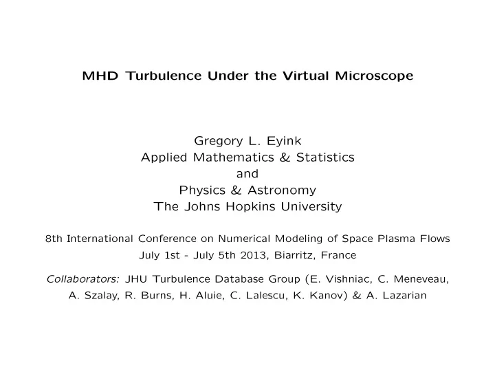
Richardson’s table of raw data Richardson’s approach was semi-empirical. By estimating “effective diffusivity” K = |∆x|2/t as a function of ℓ =

  • |∆x|2, he found from

data that K(ℓ) ∼ K0ℓ4/3. He proposed that the probability density func- tion of the separation vector ℓ = x1−x2 would satisfy a diffusion equation ∂tP(ℓ, t) = ∂ ∂ℓi

  • K(ℓ)∂P

∂ℓi (ℓ, t)

  • with scale-dependent 2-particle eddy-diffusivity.

This equation predicts at long times that |x1(t) − x2(t)|2 ∼ t3, averaging over velocity realizations.

slide-19
SLIDE 19

Similarity Solution Richardson (1926) observed that there is an exact similarity so- lution of his equation, given by the stretched-exponential PDF P∗(ℓ, t) = A (K0t)9/2 exp

  • −9ℓ2/3

4K0t

  • in three space dimensions. All solutions approach this self-similar

form asymptotically at long times. Averaging ℓ2 with respect to this density yields ℓ2(t) = γ0t3 with γ0 = 1144K3

0/81.

slide-20
SLIDE 20

Kolmogorov Cascade Picture

A cartoon of the Kolmogorov cascade In the Kolmogorov (1941) picture, velocity differences across eddies of size ℓ have mag- nitude δu(ℓ) ∼ (εℓ)1/3. This increases with ℓ, so that larger turbulent eddies have larger velocities. A pair of particles as they separate thus expe- rience greater relative velocities as they move further apart. The outcome is an explosive separation ℓ2(t) ∼ g0εt3, even much faster than ballistic (∝ t2). The (presumed universal) constant g0 is now usually called “Richardson’s constant”.

slide-21
SLIDE 21

Advection by Kolmogorov Velocity A toy calculation: Assume that ℓ(t) satisfies d dtℓ(t) = δu(ℓ) = 3 2(g0εℓ)1/3. Separation of variables gives the exact solution ℓ(t) =

  • ℓ2/3

+ (g0ε)1/3(t − t0)

3/2

. For t − t0 ≫ ℓ2/3 /(g0ε)1/3 ≡ T0 ℓ2(t) ∼ g0εt3. The condition for this behavior, δu(ℓ) ∝ ℓ1/3, is equivalent to the Kolmogorov energy spectrum E(k) ∝ k−5/3 which is very common in astrophysical plasmas.

slide-22
SLIDE 22

Advection by Kolmogorov Velocity A toy calculation: Assume that ℓ(t) satisfies d dtℓ(t) = δu(ℓ) = 3 2(g0εℓ)1/3. Separation of variables gives the exact solution ℓ(t) =

  • ℓ2/3

+ (g0ε)1/3(t − t0)

3/2

. ⇐ = This is odd!! For t − t0 ≫ ℓ2/3 /(g0ε)1/3 ≡ T0 ℓ2(t) ∼ g0εt3. The condition for this behavior, δu(ℓ) ∝ ℓ1/3, is equivalent to the Kolmogorov energy spectrum E(k) ∝ k−5/3 which is very common in astrophysical plasmas.

slide-23
SLIDE 23

Fate of Particles Initially at the Same Point? The odd feature of the previous result is that, if ℓ0 = 0, then ℓ2(t) = g0ε(t − t0)3 > 0. Two particles started at the same point at time t0 separate to a finite distance at any time t > t0! The same oddity may be seen in Richardson’s similarity solution, which satisfies at initial time t0 = 0 P∗(ℓ, 0) = δ3(ℓ). All particles start with separation ℓ(0) = 0. However, P∗(ℓ, t) is a smooth density for t > 0, so that ℓ(t) > 0 with probability one.

slide-24
SLIDE 24

Breakdown of Laplacian Determinism According to Richardson’s results, Lagrangian fluid particles that are advected by the fluid velocity u(x, t) starting at x0 d dtx(t) = u(x(t), t),

x(t0) = x0

have the property that there is more than one solution. Doesn’t this violate the theorem on uniqueness of solutions of initial-value problems for ODE’s? No! Loophole: The theorem requires that u(x, t) be x−differentiable. A turbulent velocity field in a Kolmogorov inertial range is only H¨

  • lder continuous

|u(x1, t) − u(x2, t)| ≤ C|x1 − x2|h with exponent h . = 1/3.

slide-25
SLIDE 25

Spontaneous Stochasticity

!2 !1 1 0.5

! x" t3/2 x0

Consider d˜

x = uν(˜ x, t)dt +

√ 2λd ˜

W(t),

˜

x(t0) = x0

where ν is a viscosity which smooths the ve-

  • locity. What happens as λ → 0 with Prandtl

number Pr = ν/λ fixed? At least in the Kazantsev-Kraichnan kinematic dynamo model there is a nontrivial limiting distribution Pu(x, t|x0, t0) over an infinite fam- ily of solutions to the (deterministic) initial- value problem ˙

x = u(x, t), x(t0) = x0.

There is an obvious analogy with spontaneous symmetry-breaking, e.g. a non-vanishing mean- magnetization in a ferromagnet even in the limit of zero external magnetic field. See Falkovich et al. Rev. Mod. Phys. (2001), Section II.C

slide-26
SLIDE 26

Spontaneous Stochasticity

!2 !1 1 0.5

! x" t3/2 x0

Consider d˜

x = uν(˜ x, t)dt +

√ 2λd ˜

W(t),

˜

x(t0) = x0

where ν is a viscosity which smooths the ve-

  • locity. What happens as λ → 0 with Prandtl

number Pr = ν/λ fixed? The distribution does not collapse! At least in the Kazantsev-Kraichnan kinematic dynamo model there is a nontrivial limiting distribution Pu(x, t|x0, t0) over an infinite fam- ily of solutions to the (deterministic) initial- value problem ˙

x = u(x, t), x(t0) = x0.

There is an obvious analogy with spontaneous symmetry-breaking, e.g. a non-vanishing mean- magnetization in a ferromagnet even in the limit of zero external magnetic field. See Falkovich et al. Rev. Mod. Phys. (2001), Section II.C

slide-27
SLIDE 27

Stochastic Flux-Freezing in MHD Turbulence

0.2 0.4 0.6 0.8 1 1.2 1.4 0.5 1 1.5 2 2.5 3 t Error for a representative point standard N= 512 N=1024 N=2048 N=4096

The stochastic flux-freezing theorem is well-satisfied in the MHD database. Despite the fact that the conductivity (or magnetic Reynolds number) is high, standard flux-freezing is not even approximately valid. (G. E. et al., Nature, 2013)

slide-28
SLIDE 28
slide-29
SLIDE 29

Stochastic Flux-Freezing in MHD Turbulence

0.2 0.4 0.6 0.8 1 1.2 1.4 0.5 1 1.5 2 2.5 3 t Error for a representative point standard N= 512 N=1024 N=2048 N=4096

The stochastic flux-freezing theorem is well-satisfied in the MHD database. Despite the fact that the conductivity (or magnetic Reynolds number) is high, standard flux-freezing is not even approximately valid. (G. E. et al., Nature, 2013)

slide-30
SLIDE 30

Does Richardson Dispersion Exist in Homogeneous MHD Turbulence?

Unlike in hydrodynamic turbulence, there are expected to be a significant effects of the Lorentz force in nonlinear MHD turbulence. Particle separations will be different parallel and perpendicular to the magnetic field. The laws of 2-particle dispersion will depend upon the theory of MHD turbulence. Assuming the generalized Boldyrev (2005) scaling δu(r⊥) ∼ vAM

2(2+α) 3+α

A

  • r⊥

Lf

  • 1

3+α

, with MA = brms/ ¯ B, one obtains from dr⊥/dt ∼ δu(r⊥) the Richardson-type law r2

⊥(t) ∼ L2 fM4 A

  • vAt

Lf

2(3+α)

2+α

, for the transverse slippage of magnetic field lines in MHD turbulence. Richardson dispersion has not yet been observed in MHD simulations, despite prior attempts:

  • A. Busse et al., “Statistics of passive tracers in three-dimensional magnetohydrodynamic

turbulence,” Phys. Plasmas 14 122303 (2007)

  • A. Busse and W.-C. M¨

uller, “Diffusion and dispersion in magnetohydrodynamic turbulence: The influence of mean magnetic fields,” Astron. Nachr. 329 714 (2008)

slide-31
SLIDE 31

Richardson Dispersion of Field-Lines Field-lines disperse through the plasma faster along the direction of the local mean magnetic field than they disperse perpendicular to the field, but the growth is the same power r2

i (t) ∼ L2 fM4 A

  • vAt

Lf

8

3

, in both directions, i = , ⊥ .This growth-law is consistent with the −3/2 energy spectra of the database flow, or h = 1/4 scaling expo- nent of velocity and magnetic fields. The standard diffusive estimate ∼ 4λt, pro- portional to microscopic plasma resistivity, is valid for only about one resistive time!

10−1 100 101 t

  • τb
  • 10−1

100 101 102 103 104 r2

i (t)ηb2

4t i = || i =⊥

slide-32
SLIDE 32

Richardson Dispersion of Field-Lines Field-lines disperse through the plasma faster along the direction of the local mean magnetic field than they disperse perpendicular to the field, but the growth is the same power r2

i (t) ∼ L2 fM4 A

  • vAt

Lf

8

3

, in both directions, i = , ⊥ . This growth-law is consistent with the −3/2 energy spectra of the database flow, or h = 1/4 scaling expo- nent of velocity and magnetic fields. The standard diffusive estimate ∼ 4λt, pro- portional to microscopic plasma resistivity, is valid for only about one resistive time!

10−3 10−2 10−1 100 t

  • Tu
  • 10−5

10−4 10−3 10−2 10−1 100 r2

i (t)Lu2

∼ t8/3 i = || i =⊥

slide-33
SLIDE 33

Richardson Dispersion of Field-Lines Field-lines disperse through the plasma faster along the direction of the local mean magnetic field than they disperse perpendicular to the field, but the growth is the same power r2

i (t) ∼ L2 fM4 A

  • vAt

Lf

8

3

, in both directions, i = , ⊥ . This growth-law is consistent with the −3/2 energy spectra of the database flow, or h = 1/4 scaling expo- nent of velocity and magnetic fields. The standard diffusive estimate ∼ 4λt, pro- portional to microscopic plasma resistivity, is valid for only about one resistive time! What you learned in the textbooks about magnetic flux-freezing for high-conductivity MHD plasmas is wrong.

10−3 10−2 10−1 100 t

  • Tu
  • 10−5

10−4 10−3 10−2 10−1 100 r2

i (t)Lu2

∼ t8/3 i = || i =⊥

slide-34
SLIDE 34

Further Evidence of Richardson Dispersion

Shown are PDFs of separation distances of field-lines, r parallel and r⊥ perpendicular to the local mean magnetic field. As expected from Richardson’s theory, the PDF’s are self-similar in time and have stretched-exponential form, roughly P(r) ∝ exp(−Cr3/4) for h = 1/4.

slide-35
SLIDE 35

Turbulent Magnetic Reconnection

Assume that the reconnection occurs in a background MHD plasma turbulence with rms velocity uL < vA and integral length or injection scale Lf > L.

Richardson diffusion of field-lines gives ∆

  • r2

⊥(tA) ∼ LfM 2 A

  • vAtA

Lf

3+α

2+α

, with tA = L/vA the Alfv´ en crossing time and MA = brms/ ¯

  • B. Mass conservation vRL = vA∆

with v0 vA yields vR = vAM 2

A(L/Lf)

1 2+α

Now Lazarian-Vishniac (1999) theory is ob- tained, for the case α = 0. The reconnection rate is independent of resistivity!

Estimating for solar flares that Lf ≃ L and MA ≃ 0.1 (Bemporad, 2008) one obtains a release time of about one hour. For more details, see Eyink, Lazarian & Vishniac, ApJ. 743 1-28 (2011)

slide-36
SLIDE 36

Selected References

Stochastic Flux-Freezing

  • G. L. Eyink, Stochastic flux-freezing and magnetic dynamo, Phys.

Rev.

  • E. 83 056405

(2011)

  • G. L. Eyink, A. Lazarian & E. T. Vishniac, Fast magnetic reconnection and spontaneous

stochasticity, Astrophys. J., 743 1-28 (2011)

  • G. L. Eyink et al. Flux-freezing breakdown in high-conductivity magnetohydrodynamic tur-

bulence, Nature, 497 466-469 (2013) JHU Turbulence Database

  • Y. Li et al., A public turbulence database cluster and applications to study Lagrangian

evolution of velocity increments in turbulence, J. Turbulence, 9, 31: 1-29 (2008)

  • H. Yu et al., Studying Lagrangian dynamics of turbulence using on-demand fluid particle

tracking in a public turbulence database, J. Turbulence, 13, 12: 1-29 (2012) http://turbulence.pha.jhu.edu