Medium edium Acces ccess Cont ontrol ol Prot otocols ocols 1 - - PDF document

SLIDE 1

1

1

CMPE 252A: Computer Networks SET 3:

Medium edium Acces ccess Cont

• ntrol
• l

Prot

• tocols
• cols

2

medium access control logical link control

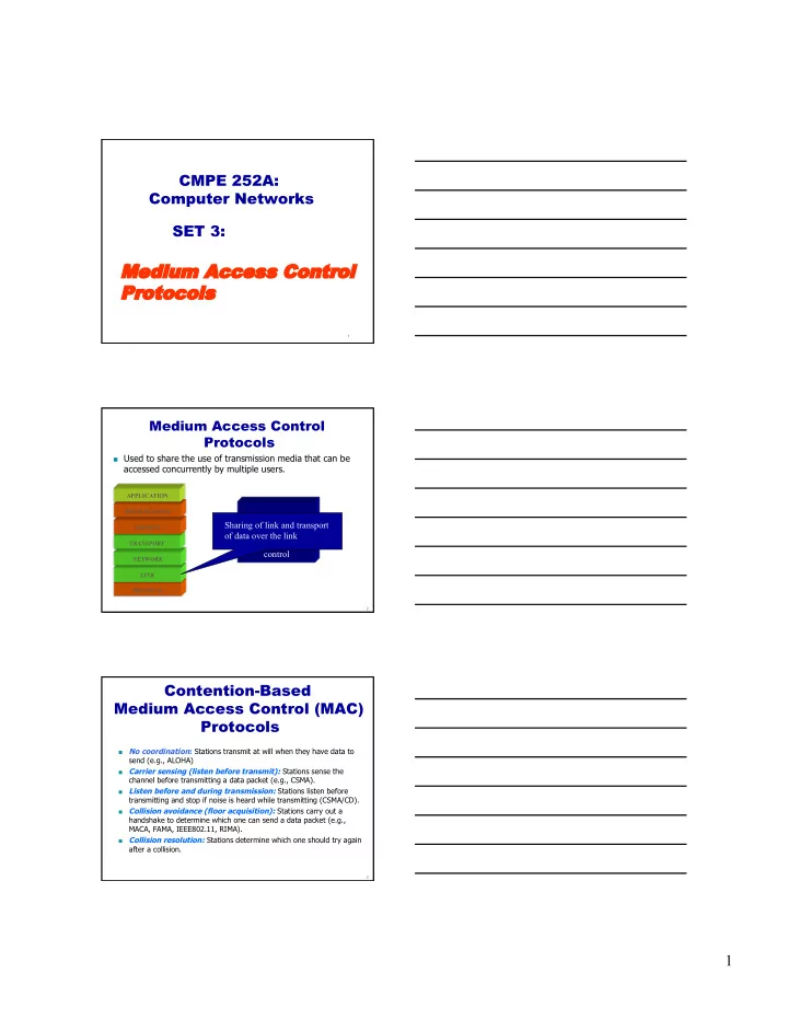
Medium Access Control Protocols

 Used to share the use of transmission media that can be

accessed concurrently by multiple users.

PHYSICAL LINK NETWORK TRANSPORT SESSION PRESENTATION APPLICATION

Sharing of link and transport

• f data over the link

3

Contention-Based Medium Access Control (MAC) Protocols



No coordination: Stations transmit at will when they have data to send (e.g., ALOHA)



Carrier sensing (listen before transmit): Stations sense the channel before transmitting a data packet (e.g., CSMA).



Listen before and during transmission: Stations listen before transmitting and stop if noise is heard while transmitting (CSMA/CD).



Collision avoidance (floor acquisition): Stations carry out a handshake to determine which one can send a data packet (e.g., MACA, FAMA, IEEE802.11, RIMA).



Collision resolution: Stations determine which one should try again after a collision.

SLIDE 2

2

4

Conflict-Free MAC Protocols

 Fixed assignment (TDMA, FDMA)  Reservations  Polling  Token passing  Dynamic transmission scheduling

 Can involve division in time, frequency or codes  Uses contention-based mechanisms to derive

transmission schedules

Aloha Tower in Honolulu, HI The ALOHA System (Norm Abramson & Frank Kuo):

Packet Switching in Radio Channels

Can You Say ALOHA?

G

Ge S

2 −

=

G S 0.18 0.5

Computer Communication Networks, Chapter 14, Prentice Hall, 1973

ALOHA Protocol

 The first protocol for multiple access channels;

and the first analysis of such protocols (Norm Abramson, Univ. of Hawaii, 1970).

 Originally planned for systems with a central base

station or a satellite transponder.

Two frequency bands; Up link and down link

(413MHz, 407MH at 9600bps)

Central node retransmits every packet it receives!

SLIDE 3

3

7

ALOHA Protocol

 Population is a large number of bursty

stations.

 Each station transmits a packet whenever it

receives it from its user; no coordination with other stations!

 Central node retransmits all packets (good

• r bad) on down link.

 Stations decide to retransmit based on the

information they hear from central node

positive ack?

8

ALOHA Protocol

An integral part of the ALOHA protocol is feedback from the receiver Feedback occurs after a packet is sent No coordination among sources

Packet ready? yes transmit yes

no

compute random backoff integer k

no

delay packet transmission k times wait for a round-trip time

9

The ALOHA Channel

 We assume:

 An (essentially) infinite population of stations.  An ideal perfect down link for the transmission of

feedback to senders.

 Stations are half duplex; have zero processing delays.  Retransmissions are scheduled such that all packets are

statistically independent.

 Each packet has the same duration P.  Stations have the same round-trip delay from one

• ther; this time can be much longer than P (irrelevant).

 Packet arrivals are Poisson with rate lambda.  Collisions are the only sources of errors.

SLIDE 4

4

10

The ALOHA Channel



What percentage of time is the channel sending correct packets? This gives us the throughput of the protocol.

time user i time user j time sum

...

NEW

NEW

P NEW

NEW

collision

I B I B I B I B I NEW RET. RET. RET. RET.

τ

Throughput of ALOHA Protocol

time

node i frame

t0

All packets have the same length

packet overlaps with start of packet from node i

t0 - 1 t0 + 1

packet overlaps with end of packet from node i

interfering frame interfering frame

Node i’s frame is vulnerable from any arrival in the time interval (t0-1, t0+1]

Throughput of ALOHA Protocol

Organize the time axis around packet from node i in terms of time slots lasting one packet length, and starting times given according to the start

• f the packet from node i.

time slot 2 time slot 1 time

node i frame

t0

packet overlaps with start of packet from node i

t0 - 1 t0 + 1

packet overlaps with end of packet from node i

interfering frame interfering frame

SLIDE 5

5

Throughput of ALOHA Protocol

time

node i frame

interfering frame interfering frame

packet overlaps with start of packet from node i packet overlaps with end of packet from node i

t0 t0 - 1 t0 + 1 The probability of a station starting a packet in a given time slot is p. Node i transmits in time slot starting at t0, i.e., time slot 2. The packet from node i is successful if no other station transmits in the time slots 1 and 2.

N nodes in the system

Throughput of ALOHA Protocol

time

node i frame

interfering frame interfering frame packet overlaps with start of packet from node i packet overlaps with end of packet from node i

t0 t0 - 1 t0 + 1 Because transmissions are independent, this means that the packet from node i succeeds with probability 1 ) 1 ( ) 1 ( ) 1 ( succeeds} node from pkt {

2

− = − = − − = N M p p p p p i P

M M M

P{a pkt succeeds} = Np (1− p)M

( )

2

Only one node can succeed, and there are C(N, 1) ways to pick the winning node; hence, the probability that any given packet that starts at time t0 succeeds is:

(a)

Throughput of ALOHA Protocol

time

node i frame

interfering frame interfering frame packet overlaps with start of packet from node i packet overlaps with end of packet from node i

t0 t0 - 1 t0 + 1 Np is the total traffic generated in a given time slot; call it G, i.e., Np = G and p = G/N The throughput of the channel is the percentage of packets offered to the channel that are successful. The throughput of the channel then equals the probability that a packet is successful, i.e., S = P{a packet succeeds}

SLIDE 6

6

Throughput of ALOHA Protocol

G

Ge S

2 −

=

Make N tend to infinity (a large user population; N~N-1 ). A useful limit is:

1

1 1 lim e x

x x

= ⎟ ⎠ ⎞ ⎜ ⎝ ⎛ +

∞ →

Making x = N , we have for a very large N: G S 0.18 0.5

S = Np (1− p)N−1

( )

2 = G

1− G N " # $ % & '

N−1

" # $ $ % & ' '

2

Substituting Np = G and p = G/N in Eq. (a) we obtain:

G 1− G N " # $ % & '

N

" # $ $ % & ' '

2

= G 1+ (−G) N " # $ % & '

N

" # $ $ % & ' '

2

→ G e−G

( )

2 = Ge−2G

Simple(r) Throughput Analysis

• f ALOHA Protocol

time

node i frame

t0

All packets have the same length Poisson arrivals with parameter λ

packet overlaps with start of packet from node i

t0 - 1 t0 + 1

packet overlaps with end of packet from node i

interfering frame interfering frame

Node i’s frame is vulnerable from any arrival in the time interval (t0-1, t0+1]

18

is the arrival rate. For convenience, we normalize the arrival rate as:

P G λ =

λ From the definition of throughput:

p G S × =

where p is the probability of a successful packet transmission Because arrivals are Poisson and all packets have equal length, every packet has the same probability of being successful. A packet is successful if no packets arrive within P seconds before it starts or while it is being transmitted; accordingly,

G P

e e p

2 ) 2 ( − −

= =

λ

Therefore, G

Ge S

2 −

=

G S 0.18 0.5

Simple(r) Throughput Analysis

• f ALOHA Protocol

SLIDE 7

7

Throughput of ALOHA Protocol

Highest throughput when we have one packet for each two-packet time period

time

node i frame

t0

packet overlaps with start of packet from node i

t0 - 1 t0 + 1

packet overlaps with end of packet from node i

interfering frame interfering frame

Node i’s frame is vulnerable from any arrival in the time interval (t0-1, t0+1]

Why Is ALOHA So Important?

 The first protocol for multiple access channels.  The first performance analysis of such protocols

(Norm Abramson, Univ. of Hawaii, 1970).

 Kleinrock and students proposed “CSMA,” which

evolved into today’s WiFi.

 Bob Metcalf proposed “CSMA/CD” (Ethernet)  Local area networking became a reality.  Led many to adopt the “independence assumption” in

the performance analysis of many protocols

21

Slotted ALOHA

 The throughput of ALOHA can be improved by reducing

the time a packet is vulnerable to interference from other packets.

 Slotted ALOHA works in a “slotted channel” providing

discrete time slots.

 Stations can start transmitting only at the beginning of

time slots.

 The time synchronization needed for slotting is

accomplished at the physical layer, and some synchronization is required in many cases anyway.

SLIDE 8

8

22

Slotted ALOHA Protocol

Packet ready? transmit yes wait for a round-trip time quantized in slots positive ack? yes

no

compute random backoff integer k

no

delay packet transmission k times Wait for start of next slot

23

Throughput of Slotted ALOHA

The vulnerability period of a packet is a slot time: Any arrivals in prior slot collide with packet i

time arrivals

i

If T is the duration of a time slot and G is the normalized packet arrival rate, then

P T Ge S Ge S

G T

= = =

− −

for ;

λ

We can obtain the same result by computing the likelihood and average length of utilization, idle and busy periods. This is the basis for a general approach to computing throughout.

24

Slotted ALOHA

...

P τ collision

time user i time user j time sum

time slot

I B I B B I B

NEW NEW NEW NEW NEW NEW RET RET

IMPORTANT: The starting point of a busy period is a “renewal point”! System is busy

SLIDE 9

9

25

Renewal Theory

 Recall the Poisson random process:  N(t) = number of arrivals in (0, t]  Inter-arrival times are exponentially distributed  N(t) is a counting process with exponential

inter-arrival times.

 Definition of Renewal Process:

A counting process N(t) for which inter-arrival

times X1, X2, …, Xn are an independent identically distributed (iid) random sequence.

26

Poisson Random Variable

A sequence of n independent Bernoulli trials;

with X being the number of arrivals in (0, t]

arrivals. 1

• r

having

• f

y probabilit the to compared negligible is in arrival

• ne

than more

• f

y probabilit The : and Make t t n Δ → Δ ∞ →

By assumption, whether or not an event occurs in a subinterval is independent of the outcomes in other subintervals. We have:

t Δ

….

time

t

arrival 1 2 3 4 n 1 2 3 k

27

Renewal Theory Example

 At each time t = 1, 2, …, a Bernoulli process

N(t) has an arrival with probability p, and this is independent of the occurrence of arrivals at any

• ther times.

 Is N(t) a renewal process?

….

time arrival 1 2 3 4 n 1 2 3 k

SLIDE 10

10

28

Renewal Theory Example

 Answer:  For any inter-arrival period n, the inter-arrival time

Xn equals x if there were x-1 Bernoulli failures followed by a success.

….

time

(1-p) (1-p) (p)

1 2 3 Xn = 3 if we have 2 failures followed by a success!

29

Renewal Theory Example

 Therefore, each inter-arrival time Xn has the Geometric

PMF:

 Because each Bernoulli trial is independent, Xn is

independent of the previous inter-arrival times X1, X2 ,…Xn-1.

 This implies that a Bernoulli arrival process is a

renewal process!

! " # = − =

−

• therwise

1,2,... x ) 1 ( ) (

1 p

p x P

x X n

30

Renewal Theory

 After an arrival (in a renewal process),

the subsequent inter-arrival times are distributed identically to the original inter-arrival times.

 Effectively, the process restarts, or has a

renewal, whenever an arrival occurs!

SLIDE 11

11

31

Renewal Theory

 Suppose that N(t) has n arrivals by time t1, the

additional time until the next arrival is denoted by Sn+1 - t1, and the subsequent inter-arrival times are Xn+2 , Xn+3 ,… and so on.

 Renewal Point: For a renewal process N(t), time t1

with N(t1) = n is a renewal point if Sn+1 - t1, Xn+2, Xn+3, … is an iid random sequence statistically identical to X1, X2, X3,…

 Every instant of time is a renewal point for a

Poisson process!

32

Renewal Theory

Alternating renewal process: System is on and off (that is, busy and idle).

time system

collision

...

success success

• ff on off on off on off ...

Y1 X1 Y2 X2 Y3 X3 Y4 ...

X1, X2, X3,…. are i.i.d. with mean E(X) Y1, Y2, Yx,…, are i.i.d. with mean E(Y) P(t) = P{system is ON at time t in steady state} = E(x)/{E(x)+E(Y)} Average cycle length = E(X) + E(Y)

33

Evaluating Throughput

 We assume that the system is “stationary,” i.e., system behaves in

cycles that are statistically equivalent

 Average cycle consists of an idle period (I ) and a busy period (B ).  The busy portion of a cycle has good and part parts.  The portion of time used to send user data is called the utilization

period (U )

Throughput is defined as: S = U I + B = U I +(P

gBg + P bBb)

time

success failure

g

B I

b

B

good busy period idle period bad busy period

SLIDE 12

12

34

Evaluating Throughput

 The expression for S amounts to simply taking averages.  What we need to do now is compute the probability that

I, B (good a bad parts), and U happen in an average cycle, and their average duration.

 Ideally, these probabilities are based on independent

events, and we can express S based on knowledge of the present state of the system.

then

• f

component each

• f
• ccurrence
• f

y probabilit and duration average the denote and Let S i P T

i i

B B I I U U

P T P T P T B I U S + = + =

35

Throughput of Slotted ALOHA

Idle, busy and utilization periods are multiples of

time slots. We need to count the time slots in each average period and we are done. Average length of idle period: I = number of slots in idle period

time

arrivals transmissions start no arrivals idle period starts

36

Idle Period in Slotted ALOHA

T

e no P some P slot

• ne

I P

λ −

− = − = = = 1 slot} in arrive pkts { 1 slot} idle in the arrive pkts { } { I has one slot:

time

there is a prior busy period

... at least one arrival!

time

I has two slots: ... at least one arrival!

no arrivals

) 1 ( 2} slot in pkts some { 1} slot in pkts no { slot} 2nd in pkts some and slot first in pkts no { } {

T T

e e P P P slots two I P

λ λ − −

− = = × = = = =

SLIDE 13

13

37

Idle Period in Slotted ALOHA

time

I has k slots: ...

no arrivals

1 k-1 k

… some arrivals

2} slot in pkts some { } 1 slot in pkts no { ... 1} slot in pkts no { slot} last in pkts some and slots 1 first in pkts no { } { P k P P k P slots k I P × − × × = − = =

P{I = k slots} = e−λT

( )

k−1(1− e−λT )

This corresponds to the Geometric r.v., and we know its average value to be 1/p, with p being the probability of success. Success now consists of ending the idle period! Therefore: ) 1 ( 1

T

e I

λ −

− =

38

Busy Period in Slotted ALOHA

 We follow the same approach:

 Solve the problem with the Geometric random variable

time

B has k slots: ...

some arrivals

1 k-1 k

… no arrivals

2} slot in pkts no { } 1 slot in pkts some { ... 1} slot in pkts some { slot} last in pkts no and slots 1 first in pkts some { } { P k P P k P slots k B P × − × × = − = =

P{B = k slots} = 1− e−λT

( )

k−1(e−λT )

T T

e e B

λ λ

= =

−

1

prior slot considered in idle period

39

Utilization Period

 Here we have to make use of conditional probability!  A busy period has good and bad time slots (transmission

periods).

collision

time sum

The probability that a slot (transmission period) in the current busy period is successful is the probability that only

• ne packet arrives in the prior slot, given that there is a

busy period Arrivals are Poisson, so we make use of the definition of that random variable as follows….

SLIDE 14

14

40

Utilization Period

T T S

e Te T some P T

• ne

P T some P T some and T

• ne

P T some T P P

λ λ

λ

− −

− = = = = 1 } in arrivals { } in arrival { } in arrivals { } in arrivals in arrival { } in arrivals | in arrival

• ne

{

The probability that a given slot within a busy period is successful is: The portion of an average busy period used to send useful data equals the length of the average busy period in slots, times the probability that any given slot is successful.

T T T T S

e T e Te e P B U

λ λ λ λ

λ λ

− − −

− = # # $ % & & ' ( − = × = 1 1

We can use the Binomial random variable to proof the above!

41

Throughput of Slotted ALOHA

 We now just substitute B,I, and U in S:

10

• 3

10

• 2

10

• 1

10 10

1

10

2

10

3

10

4

10

5

0.1 0.2 0.3 0.4 0.5 0.6 0.7 0.8 0.9 1 Analytical Results Offered Load: G S (Throughput) Pure CSMA Slotted CSMA Pure Aloha Slotted Aloha

T T T T

Te e e e T B I U S

λ λ λ λ

λ λ

− − −

= + − # $ % & ' ( − = + = 1 1 1 1

Maximum throughput is twice that of ALOHA. This occurs when G = 1

T G with Ge S

G

λ = =

−

42

Average Delay of MAC Protocols

 We want to measure or compute the average time

from the instant the first bit of a packet is first transmitted to the moment the last bit is received correctly at the destination.

 Assume that arrivals (of new and retransmitted

data or control packets) to the channel are Poisson.

 Assume fully-connected networks.

SLIDE 15

15

43

Average Delay in ALOHA

Direct method: The average number of transmissions needed for a packet to be received correctly is

G

e S G

2

/ =

Therefore, the number of retransmissions is

1 1 /

2 −

= −

G

e S G

Assumptions: A satellite channel with propagation delay NxP, where P is the packet length and NxP >> P A retransmission is sent after an average backoff time of BxP seconds. A packet is transmitted (G/S-1) times in error (due to collisions) and each such transmission wastes P+NxP +BxP seconds. The last transmission is successful and must take P+NxP seconds. Therefore, the average delay incurred is:

) )( 1 (

2

P B P N P e P N P D

G

× + × + − + × + =

44

Average Delay in ALOHA

Indirect Method: Based on the fact that the success of a transmission is independent of

• thers, and knowing how many times we have retransmitted does not

change the likelihood of success in the next transmission! We use a diagram showing possible states, probabilities of transition, and delay incurred in that transition.

START END BACK OFF

P N P , × +

S

P P B P N P , 1 × + × + −

S

P P B P N P , 1 × + × + −

S

P P N P , × +

S

P From the diagram. we obtain a number of simultaneous equations that we solve to obtain delay from START to END.

45

Average Delay in ALOHA

From the diagram we have:

) )( 1 ( ) ( R P B P N P P P N P P D

S S

+ × + × + − + × + = ) )( 1 ( ) ( R P B P N P P P N P P R

S S

+ × + × + − + × + =

Solving these two equations:

) ( ) 1 ( P B P N P P P P N P R

S S

× + × + − + × + = ) )( 1 (

1

P B P N P P P N P D

S

× + × + − + × + =

−

Substituting

G S

e P

2 −

=

we obtain the same result expected from the Geometric r.v. The same method can be applied on the other MAC protocols!

SLIDE 16

16

46

Average Delay of ALOHA

 The delay increases exponentially with heavy load, which

is not acceptable for real-time applications.

47

CSMA: Carrier Sense Multiple Access

 The capacity of ALOHA or slotted ALOHA is limited

by the large vulnerability period of a packet.

 By listening before transmitting, stations try to

reduce the vulnerability period to one propagation delay.

 This is the basis of CSMA (Kleinrock and Tobagi,

UCLA, 1975)

 Many of the assumptions made for ALOHA are

made now for CSMA.

48

CSMA Protocol

Assume non-persistent carrier sensing. Requires a maximum propagation delay much smaller than packet lengths!

transmit no wait for a round-trip time positive ack? yes compute random backoff integer k

no

delay packet transmission k times Packet ready Channel Busy? yes

SLIDE 17

17

49

CSMA Throughput

A virtual secondary channel used to send ACKs reliable and in 0 time! Same assumptions made for pure ALOHA analysis. All stations are at one propagation delay from each other and that equals:

τ

Arrivals are Poisson with average rate λ Peer-to-peer communication No base station or transponder Explicit feedback to sender!

50

CSMA Protocol

The big difference compared to ALOHA is that busy periods are bounded!

time user i time user j time sum

...

I B I B I B I RET. RET. RET RET

NEW

NEW

P NEW

NEW

collision

τ 2 + ≤ P B

τ

51

CSMA Throughput

P

time RET. RET.

NEW

NEW

collision

τ

I B I B I B I

τ 2 + ≤ P

failed period

τ + P

successful period

Length of average idle period (exponential interarrivals)?

λ / 1 = I

The probability that a packet is successful is?

λτ −

= e P

S

The average length of a utilization period is? (no packets can arrive within tau sec. after the start of the packet!)

λτ −

× = e P U

We can approximate:

τ 2 + = P B

SLIDE 18

18

52

CSMA Throughput

Substituting we have: λ τ

λτ

1 2 + + ≈

−

P Pe S Pretty accurate for << P More accurate estimation of S requires finding the average length of B.

time

FIRST LAST

P

START END

Y Y

Y is a random variable!

τ + + = Y P B

τ τ τ

53

CSMA Throughput

) (

) sec in arrivals ( ) ( ) (

y Y

e y P y F y Y P

− −

= − = = ≤

τ λ

τ

time

FIRST LAST START

Y =y

no arrivals, no more arrivals occur after LAST

y − τ

) 1 ( 1 ) 1 ( )) ( 1 ( ) (

) ( λτ τ τ λ

λ τ

− − − ∞

− − = + − = − =

∫ ∫

e dy e dy y F Y E

y Y

) 1 ( 1 2

λτ

λ τ

−

− − + = e P B

Note that the average length of B is determined by the time between the start

• f the first and the last packet in the busy

period.

τ

54

CSMA Throughput

Substituting we get:

10

• 3

10

• 2

10

• 1

10 10

1

10

2

10

3

10

4

10

5

0.1 0.2 0.3 0.4 0.5 0.6 0.7 0.8 0.9 1 Analytical Results Offered Load: G S (Throughput) Pure CSMA Slotted CSMA Pure Aloha Slotted Aloha

aG aG

e G a Ge S

− −

+ + = ) 2 1 (

P a P G / , with τ λ = =

S = Ge−aG (1+ 2a)G +1

Approximate:

SLIDE 19

19

55

Slotted CSMA



Non-persistent strategy.



A slot lasts one maximum propagation delay.

no wait for a round-trip time quantized in slots positive ack? yes compute random backoff integer k

no

delay packet transmission k times Packet ready Channel Busy? yes transmit

wait for start of next slot

56

Computing the Throughput of Slotted CSMA

NEW

P

time

collision

τ

I B I B I

success

RET. time

I has k slots: ...

no arrivals

1 k-1 k

… some arrivals

Just as in slotted ALOHA, with slot duration equal to

τ τ

sec ) 1 ( ; slots ) 1 ( 1

λτ λτ

τ

− −

− = − = e I e I

57

Throughput of Slotted CSMA

 We follow the same approach as in slotted ALOHA  B has k transmission periods, each of P + τ sec  What happens in a transmission period depends only on the

last time slot of the prior transmission period! P{B = k trans. periods} = P{B = k(P +τ) sec} = 1− e−λτ

( )

k−1(e−λτ )

time

...

some arrivals in last slot of each transmission period

1 k-1 k

… no arrivals in last slot of

last transmission period

τ + P

Slotted CSMA:

SLIDE 20

20

58

Throughput of Slotted CSMA

sec ) (

λτ λτ

τ τ e P e P B + = + =

−

so , 1 } in arrivals { } in arrival {

λτ λτ

λτ τ τ

− −

− = = e e some P

• ne

P P

S

sec

S

P P B P U × + × = τ

A transmission period is successful with probability and the period has useful data for P seconds

S

P sec 1

λτ

λτ

−

− = e P U

periods ion transmiss 1

λτ −

= e B

We use the Geometric r.v. to

• btain the average number of

transmission periods in B :

59

Throughput of Slotted CSMA

 We now substitute U, B and I in S:

P a P G e a aGe S

aG aG

/ , with ; ) 1 ( τ λ = = − + =

− −

60

CSMA Throughput

 Because prop. delay is much smaller than pkt length, slotted

and pure CSMA have very similar performance.

 When MAC protocol requires small prop delays, we

can use slotted version to predict performance of unslotted version.

10

• 3

10

• 2

10

• 1

10 10

1

10

2

10

3

10

4

10

5

0.1 0.2 0.3 0.4 0.5 0.6 0.7 0.8 0.9 1 Analytical Results Offered Load: G S (Throughput) Pure CSMA Slotted CSMA Pure Aloha Slotted Aloha

Reminder: These results are

• nly an upper bound on

performance, because we did not take into account the effect of ACKs sent from receivers!

SLIDE 21

21

61

CSMA/CD: CSMA with Collision Detection

 CSMA improves on the performance of ALOHA

tremendously.

 The remaining limitation is that, once a packet is sent,

feedback occurs a roundtrip time after the entire packet is transmitted.

 The solution to improve on the performance of CSMA is to

listen to the channel while a packet is being sent.

 This is called collision detection.



R.M Metcalfe and D.R. Boggs, “Ethernet: Distributed Packet Switching for Local Computer Networks,” Comm. ACM, Vol. 19, 1976 (Xerox PARC).

62

CSMA/CD Protocol

Non-persistent transmission strategy Collision detection serves as a NACK!

transmit no abort transmission Collision detected? no compute random backoff integer k

yes

delay packet transmission k times Packet ready Channel busy? yes send jamming signal

Assumption are:

• All stations hear one

another

• Propagation delay is much

smaller than packets Station listens to channel while transmitting; Collision is detected when signals sent and heard differ. Jamming signal sent to ensure all stations know of the collision.

63

Throughput of CSMA/CD

time

J J Z C + ≤ + + = τ τ 3 2

collision interval: successful packet:

τ + P

first packet starts (A)

τ τ τ ≤ Z J

first interfering packet starts (B) A starts hearing B and jams B starts hearing A and jams

idle period

τ

P

NEW A B

τ τ + + J

average idle period:

λ / 1 = I

) ( e 2 e ; with ) ( ] 2 )[ 1 (

• τ

τ τ τ τ

λτ λτ

− − + + + = = ≤ + + + + + − = J P J Z B P Z P Z P J Z P B

S S S

SLIDE 22

22

64

Throughput of CSMA/CD

 Notes:

 The average length of a bad busy period is much smaller than in

CSMA because J<<P.

 This length is determined by the time between the first packet in

the busy period and the first packet that interferes (in contrast, in CSMA, it is the last interfering packet that counts) For However, we can derive an exact value of the average value of Z.

P << τ

we can approximate:

) ( 3 τ τ

λτ

− − + + ≈

−

J P e J B

The utilization period is only that portion of a packet transmission that has no overhead, that is:

λτ −

= Pe U

65

Throughput of CSMA/CD

Substituting we get:

) ( 3 1 τ τ λ

λτ λτ

− − + + + ≈

− −

J P e J Pe S

66

Throughput of CSMA/CD

λτ τ λ λ λτ τ λ λ

τ τ τ τ τ τ

− − − − − − −

− − = − − = = = > = > ≤ ≤ > − = ≤ = e e e e e e P z P z P P z P z Z P z P z Z P z z Z P z Z P z F

z z z Z

1 1 ) 1 ( )} , ( in arrivals some { )} , ( in arrivals some { )} , ( in arrivals no { )} , ( in arrivals some { )} , ( in arrivals some and ) , ( in arrivals no { } { )} , ( in arrivals some | ) , ( in arrivals no { } { for }; { 1 } { ) (

) ( ) (

Therefore:

λτ λ λτ λτ λ − − − − −

− − = − − − = > − = e e e e e z Z P z F

z z Z

1 1 1 1 } { 1 ) ( ! " # $ % & − − + = − =

− −

∫

λτ λτ τ

λτ τ e e dt t F Z E

Z

1 1 2 )) ( 1 ( ) (