Maxent Models, Conditional Introduction Estimation, and - - PDF document

SLIDE 1

1 Maxent Models, Conditional Estimation, and Optimization

Dan Klein and Chris Manning Stanford University http://nlp.stanford.edu/

HLT-NAACL 2003 and ACL 2003 Tutorial

Without Magic

That is, With Math!

Introduction

In recent years there has been extensive use

• f conditional or discriminative probabilistic

models in NLP, IR, and Speech

Because:

They give high accuracy performance They make it easy to incorporate lots of

linguistically important features

They allow automatic building of language

independent, retargetable NLP modules

Joint vs. Conditional Models

Joint (generative) models place probabilities over

both observed data and the hidden stuff (gene- rate the observed data from hidden stuff):

All the best known StatNLP models:

n-gram models, Naive Bayes classifiers, hidden

Markov models, probabilistic context-free grammars

Discriminative (conditional) models take the data

as given, and put a probability over hidden structure given the data:

Logistic regression, conditional loglinear models,

maximum entropy markov models, (SVMs, perceptrons)

P(c,d) P(c|d)

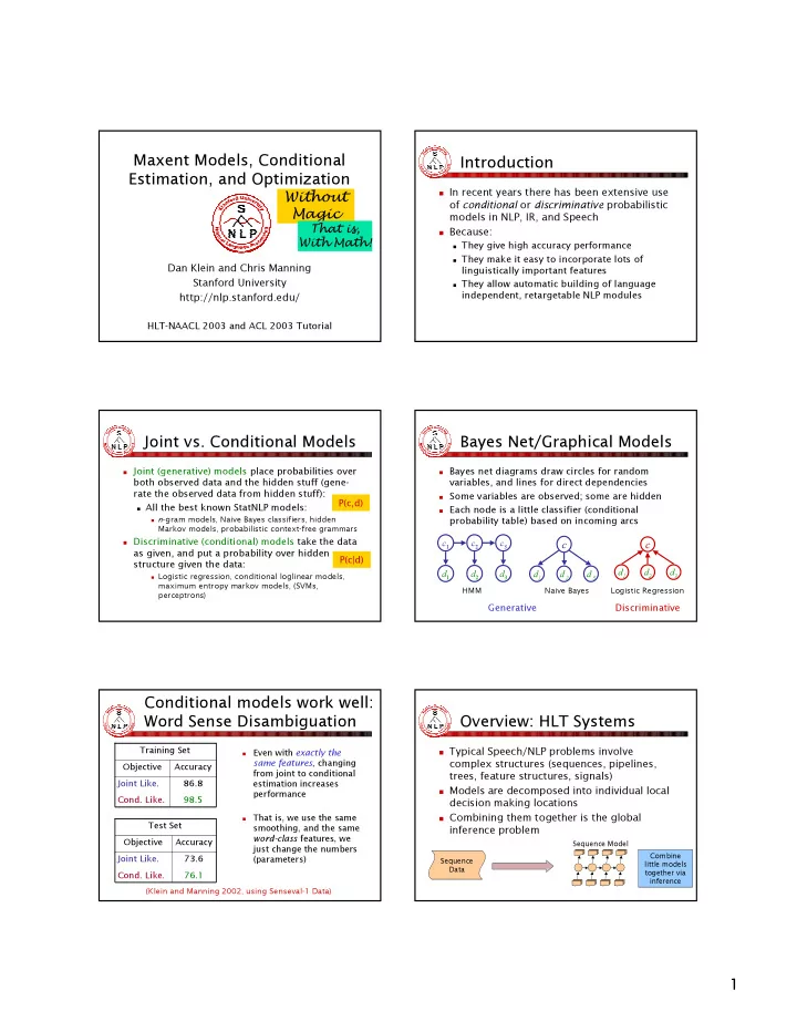
Bayes Net/Graphical Models

Bayes net diagrams draw circles for random

variables, and lines for direct dependencies

Some variables are observed; some are hidden Each node is a little classifier (conditional

probability table) based on incoming arcs c1 c2 c3 d1 d2 d3

HMM

c

d1 d 2 d 3

Naive Bayes

c

d1 d2 d3 Generative

Logistic Regression

Discriminative

Conditional models work well: Word Sense Disambiguation

Even with exactly the

same features, changing from joint to conditional estimation increases performance

That is, we use the same

smoothing, and the same word-class features, we just change the numbers (parameters) Training Set 98.5

• Cond. Like.

86.8 Joint Like. Accuracy Objective Test Set 76.1

• Cond. Like.

73.6 Joint Like. Accuracy Objective

(Klein and Manning 2002, using Senseval-1 Data)

Overview: HLT Systems

Typical Speech/NLP problems involve

complex structures (sequences, pipelines, trees, feature structures, signals)

Models are decomposed into individual local

decision making locations

Combining them together is the global

inference problem

Sequence Data Sequence Model Combine little models together via inference

SLIDE 2

2 Overview: The Local Level

Sequence Level Local Level

Local Data Feature Extraction

Features Label

Optimization Smoothing Classifier Type

Features Label

Sequence Data Maximum Entropy Models Quadratic Penalties Conjugate Gradient Sequence Model NLP Issues Inference Local Data Local Data

Tutorial Plan

• 1. Exponential/Maximum entropy models
• 2. Optimization methods
• 3. Linguistic issues in using these models

Part I: Maximum Entropy Models

• a. Examples of Feature-Based Modeling
• b. Exponential Models for Classification
• c. Maximum Entropy Models
• d. Smoothing

We will use the term “maxent” models, but will introduce them as loglinear or exponential models, deferring the interpretation as “maximum entropy models” until later.

Features

In this tutorial and most maxent work:

features are elementary pieces of evidence that link aspects of what we observe d with a category c that we want to predict.

A feature has a real value: f: C × D → R Usually features are indicator functions of

properties of the input and a particular class (every one we present is). They pick out a subset.

fi(c, d) ≡ [Φ(d) ∧ c = ci]

[Value is 0 or 1]

We will freely say that Φ(d) is a feature of the data

d, when, for each ci, the conjunction Φ(d) ∧ c = ci is

a feature of the data-class pair (c, d).

Features

For example: f1(c, d) ≡ [c= “NN” ∧ islower(w0) ∧ ends(w0, “d”)] f2(c, d) ≡ [c = “NN” ∧ w-1 = “to” ∧ t-1 = “TO”] f3(c, d) ≡ [c = “VB” ∧ islower(w0)] Models will assign each feature a weight Empirical count (expectation) of a feature: Model expectation of a feature:

TO NN to aid IN JJ in blue TO VB to aid IN NN in bed

∑

∈

=

) , (

• bserved

) , (

) , ( ) ( empirical

D C d c i i

d c f f E

∑

∈

=

) , ( ) , (

) , ( ) , ( ) (

D C d c i i

d c f d c P f E

Feature-Based Models

The decision about a data point is based

• nly on the features active at that point.

BUSINESS: Stocks hit a yearly low … Data Features {…, stocks, hit, a, yearly, low, …} Label BUSINESS Text Categorization … to restructure bank:MONEY debt. Data Features {…, P=restructure, N=debt, L=12, …} Label MONEY Word-Sense Disambiguation DT JJ NN … The previous fall … Data Features {W=fall, PT=JJ PW=previous} Label NN POS Tagging

SLIDE 3

3 Example: Text Categorization

(Zhang and Oles 2001)

Features are a word in document and class (they

do feature selection to use reliable indicators)

Tests on classic Reuters data set (and others) Naïve Bayes: 77.0% F1 Linear regression: 86.0% Logistic regression: 86.4% Support vector machine: 86.5% Emphasizes the importance of regularization

(smoothing) for successful use of discriminative methods (not used in most early NLP/IR work)

Example: NER

(Klein et al. 2003; also, Borthwick 1999, etc.)

• Sequence model across words
• Each word classified by local model
• Features include the word, previous

and next words, previous classes, previous, next, and current POS tag, character n-gram features and shape of word

Best model had > 800K features

• High (> 92% on English devtest set)

performance comes from combining many informative features.

• With smoothing / regularization,

more features never hurt! Xx Xx x Sig NNP NNP IN Tag Road Grace at Word ??? ??? Other Class Next Cur Prev

Local Context

Decision Point: State for Grace

Example: NER

0.37 0.68 O-Xx Prev state, cur sig 0.37

• 0.69

x-Xx-Xx Prev-cur-next sig 2.68

• 0.58

Total: … 0.82

• 0.20

O-x-Xx

• P. state - p-cur sig

0.46 0.80 Xx Current signature

• 0.92
• 0.70

Other Previous state 0.14

• 0.10

IN NNP Prev and cur tags 0.45 0.47 NNP Current POS tag

• 0.04

0.45 <G Beginning bigram 0.00 0.03 Grace Current word 0.94

• 0.73

at Previous word LOC PERS Feature Feature Type Xx Xx x Sig NNP NNP IN Tag Road Grace at Word ??? ??? Other Class Next Cur Prev

Local Context Feature Weights

(Klein et al. 2003) Decision Point: State for Grace

Example: Tagging

Features can include: Current, previous, next words in isolation or together. Previous (or next) one, two, three tags. Word-internal features: word types, suffixes, dashes, etc.

% 22.6 fell Dow The ??? ??? VBD NNP DT +1

• 1
• 2
• 3

Local Context Features

true hasDigit? … … NNP-VBD T-1-T-2 VBD T-1 fell W-1 % W+1 22.6 W0

Decision Point

(Ratnaparkhi 1996; Toutanova et al. 2003, etc.)

Other Maxent Examples

Sentence boundary detection (Mikheev 2000)

Is period end of sentence or abbreviation?

PP attachment (Ratnaparkhi 1998)

Features of head noun, preposition, etc.

Language models (Rosenfeld 1996)

P(w0|w-n,…,w-1). Features are word n-gram

features, and trigger features which model repetitions of the same word.

Parsing (Ratnaparkhi 1997; Johnson et al. 1999, etc.)

Either: Local classifications decide parser

actions or feature counts choose a parse.

Conditional vs. Joint Likelihood

We have some data {(d, c)} and we want to place

probability distributions over it.

A joint model gives probabilities P(d,c) and tries

to maximize this likelihood.

It turns out to be trivial to choose weights:

just relative frequencies.

A conditional model gives probabilities P(c|d). It

takes the data as given and models only the conditional probability of the class.

We seek to maximize conditional likelihood. Harder to do (as we’ll see…) More closely related to classification error.

SLIDE 4

4 Feature-Based Classifiers

“Linear” classifiers: Classify from features sets {fi} to classes {c}. Assign a weight λi to each feature fi. For a pair (c,d), features vote with their weights:

vote(c) = Σλifi(c,d) Choose the class c which maximizes Σλifi(c,d) = VB There are many ways to chose weights Perceptron: find a currently misclassified example, and

nudge weights in the direction of a correct classification TO NN to aid TO VB to aid 1.2 –1.8 0.3

Feature-Based Classifiers

Exponential (log-linear, maxent, logistic, Gibbs) models: Use the linear combination Σλifi(c,d) to produce a

probabilistic model:

P(NN|to, aid, TO) = e1.2e–1.8/(e1.2e–1.8 + e0.3) = 0.29 P(VB|to, aid, TO) = e0.3 /(e1.2e–1.8 + e0.3) = 0.71

The weights are the parameters of the probability

model, combined via a “soft max” function

Given this model form, we will choose parameters

{λi} that maximize the conditional likelihood of the data according to this model.

∑ ∑

'

) , ' ( exp

c i i i

d c f λ = ) , | ( λ d c P

∑

i i i

d c f ) , ( exp λ

Makes votes positive. Normalizes votes.

Other Feature-Based Classifiers

The exponential model approach is one way of

deciding how to weight features, given data.

It constructs not only classifications, but

probability distributions over classifications.

There are other (good!) ways of discriminating

classes: SVMs, boosting, even perceptrons – though these methods are not as trivial to interpret as distributions over classes.

We’ll see later what maximizing the conditional

likelihood according to the exponential model has to do with entropy.

Exponential Model Likelihood

Maximum Likelihood (Conditional) Models :

Given a model form, choose values of

parameters to maximize the (conditional) likelihood of the data.

Exponential model form, for a data set (C,D):

∑ ∑

∈ ∈

= =

) , ( ) , ( ) , ( ) , (

log ) , | ( log ) , | ( log

D C d c D C d c

d c P D C P λ λ

∑ ∑

'

) , ' ( exp

c i i i

d c f λ

∑

i i i

d c f ) , ( exp λ

Building a Maxent Model

Define features (indicator functions) over data

points.

Features represent sets of data points which are

distinctive enough to deserve model parameters.

Usually features are added incrementally to “target”

errors.

For any given feature weights, we want to be able to

calculate:

Data (conditional) likelihood Derivative of the likelihood wrt each feature weight

Use expectations of each feature according to the model

Find the optimum feature weights (next part).

The Likelihood Value

• The (log) conditional likelihood is a function of the iid data

(C,D) and the parameters λ:

• If there aren’t many values of c, it’s easy to calculate:
• We can separate this into two components:
• The derivative is the difference between the derivatives of each component

∑ ∏

∈ ∈

= =

) , ( ) , ( ) , ( ) , (

) , | ( log ) , | ( log ) , | ( log

D C d c D C d c

d c P d c P D C P λ λ λ

∑

∈

=

) , ( ) , (

log ) , | ( log

D C d c

D C P λ

∑ ∑

'

) , ( exp

c i i i

d c f λ

∑

i i i

d c f ) , ( exp λ

∑ ∑ ∑

∈ ) , ( ) , ( '

) , ' ( exp log

D C d c c i i i

d c f λ

∑ ∑

∈ ) , ( ) , (

) , ( exp log

D C d c i i i

d c f λ − = ) , | ( log λ D C P

) (λ N ) (λ M = ) , | ( log λ D C P −

SLIDE 5

5 The Derivative I: Numerator

i D C d c i i i

d c f λ λ ∂ ∂ =

∑ ∑

∈ ) , ( ) , (

) , (

∑ ∑

∈

∂ ∂ =

) , ( ) , (

) , (

D C d c i i i i

d c f λ λ

∑

∈

=

) , ( ) , (

) , (

D C d c i

d c f

i D C d c i i ci i

d c f N λ λ λ λ ∂ ∂ = ∂ ∂

∑ ∑

∈ ) , ( ) , (

) , ( exp log ) ( Derivative of the numerator is: the empirical count(fi, c)

The Derivative II: Denominator

i D C d c c i i i i

d c f M λ λ λ λ ∂ ∂ = ∂ ∂

∑ ∑ ∑

∈ ) , ( ) , ( '

) , ' ( exp log ) (

∑ ∑ ∑ ∑ ∑

∈

∂ ∂ =

) , ( ) , ( ' ' '

) , ' ( exp ) , ' ' ( exp 1

D C d c i c i i i c i i i

d c f d c f λ λ λ

∑ ∑ ∑ ∑ ∑ ∑

∈

∂ ∂ =

) , ( ) , ( ' ' '

) , ' ( 1 ) , ' ( exp ) , ' ' ( exp 1

D C d c c i i i i i i i c i i i

d c f d c f d c f λ λ λ λ

i i i i D C d c c c i i i i i i

d c f d c f d c f λ λ λ λ ∂ ∂ =

∑ ∑ ∑∑ ∑ ∑

∈

) , ' ( ) , ' ' ( exp ) , ' ( exp

) , ( ) , ( ' ' '

∑ ∑

∈

=

) , ( ) , ( '

) , ' ( ) , | ' (

D C d c i c

d c f d c P λ

= predicted count(fi, λ)

The Derivative III

The optimum parameters are the ones for which

each feature’s predicted expectation equals its empirical expectation. The optimum distribution is:

Always unique (but parameters may not be unique) Always exists (if features counts are from actual data). Features can have high model expectations

(predicted counts) either because they have large weights or because they occur with other features which have large weights.

= ∂ ∂

i

D C P λ λ) , | ( log ) , ( count actual C fi ) , ( count predicted λ

i

f −

Summary so far

We have a function to optimize: We know the function’s derivatives: Perfect situation for general optimization (Part II) But first … what has all this got to do with

maximum entropy models?

∑

∈

=

) , ( ) , (

log ) , | ( log

D C d c

D C P λ

∑ ∑

'

) , ( exp

c i i i

d c f λ

∑

i i i

d c f ) , ( exp λ

= ∂ ∂

i

D C P λ λ / ) , | ( log ) , ( count actual C fi ) , ( count predicted λ

i

f −

Maximum Entropy Models

An equivalent approach:

Lots of distributions out there, most of them

very spiked, specific, overfit.

We want a distribution which is uniform

except in specific ways we require.

Uniformity means high entropy – we can

search for distributions which have properties we desire, but also have high entropy.

(Maximum) Entropy

Entropy: the uncertainty of a distribution. Quantifying uncertainty (“surprise”):

Event

x

Probability

px

“Surprise”

log(1/px)

Entropy: expected surprise (over p):

∑

− =

x x x

p p p log ) ( H       =

x p

p E p 1 log ) ( H

A coin-flip is most uncertain for a fair coin.

pHEADS H

SLIDE 6

6 Maxent Examples I

• What do we want from a distribution?

Minimize commitment = maximize entropy. Resemble some reference distribution (data).

• Solution: maximize entropy H, subject to

feature-based constraints:

• Adding constraints (features):

Lowers maximum entropy Raises maximum likelihood of data Brings the distribution further from uniform Brings the distribution closer to data

[ ] [ ]

i p i p

f E f E

ˆ

=

∑

∈

=

i

f x i x

C p

Unconstrained, max at 0.5 Constraint that

pHEADS = 0.3

Maxent Examples II

H(pH pT,) pH + pT = 1 pH = 0.3

• x log x

1/e

Maxent Examples III

Lets say we have the following event space: … and the following empirical data: Maximize H: … want probabilities: E[NN,NNS,NNP,NNPS,VBZ,VBD] = 1

VBD VBZ NNPS NNP NNS NN

1/e 1/e 1/e 1/e 1/e 1/e 1/6 1/6 1/6 1/6 1/6 1/6 1 3 13 11 5 3

Maxent Examples IV

• Too uniform!
• N* are more common than V*, so we add the feature fN = {NN,

NNS, NNP, NNPS}, with E[fN] =32/36

• … and proper nouns are more frequent than common nouns,

so we add fP = {NNP, NNPS}, with E[fP] =24/36

• … we could keep refining the models, e.g. by adding a feature

to distinguish singular vs. plural nouns, or verb types.

2/36 2/36 8/36 8/36 8/36 8/36 2/36 2/36 12/36 12/36 4/36 4/36

VBD VBZ NNPS NNP NNS NN

Feature Overlap

Maxent models handle overlapping features well. Unlike a NB model, there is no double counting!

1 2 b 1 2 B a A 1/4 1/4 b 1/4 1/4 B a A Empirical All = 1 b B a A 1/6 1/3 b 1/6 1/3 B a A A = 2/3 b B a A 1/6 1/3 b 1/6 1/3 B a A A = 2/3 b B a A b B a A λA b λA B a A

λ’A+λ’’A

b

λ’A+λ’’A

B a A

Example: NER Overlap

0.37 0.68 O-Xx Prev state, cur sig 0.37

• 0.69

x-Xx-Xx Prev-cur-next sig 2.68

• 0.58

Total: … 0.82

• 0.20

O-x-Xx

• P. state - p-cur sig

0.46 0.80 Xx Current signature

• 0.92
• 0.70

Other Previous state 0.14

• 0.10

IN NNP Prev and cur tags 0.45 0.47 NNP Current POS tag

• 0.04

0.45 <G Beginning bigram 0.00 0.03 Grace Current word 0.94

• 0.73

at Previous word LOC PERS Feature Feature Type Xx Xx x Sig NNP NNP IN Tag Road Grace at Word ??? ??? Other State Next Cur Prev

Local Context Feature Weights

Grace is correlated with PERSON, but does not add much evidence on top of already knowing prefix features.

SLIDE 7

7 Feature Interaction

Maxent models handle overlapping features well, but

do not automatically model feature interactions.

1 b 1 1 B a A 1/4 1/4 b 1/4 1/4 B a A Empirical All = 1 b B a A 1/6 1/3 b 1/6 1/3 B a A A = 2/3 b B a A 1/9 2/9 b 2/9 4/9 B a A B = 2/3 b B a A b B a A λA b λA B a A λA b λB

λA+λB

B a A

Feature Interaction

If you want interaction terms, you have to add them: A disjunctive feature would also have done it (alone):

1 b 1 1 B a A Empirical 1/6 1/3 b 1/6 1/3 B a A A = 2/3 b B a A 1/9 2/9 b 2/9 4/9 B a A B = 2/3 b B a A 1/3 b 1/3 1/3 B a A AB = 1/3 b B a A b B a A 1/3 b 1/3 1/3 B a A

Feature Interaction

For loglinear/logistic regression models in

statistics, it is standard to do a greedy stepwise search over the space of all possible interaction terms.

This combinatorial space is exponential in

size, but that’s okay as most statistics models only have 4–8 features.

In NLP, our models commonly use hundreds

• f thousands of features, so that’s not okay.

Commonly, interaction terms are added by

hand based on linguistic intuitions.

Example: NER Interaction

0.37 0.68 O-Xx Prev state, cur sig 0.37

• 0.69

x-Xx-Xx Prev-cur-next sig 2.68

• 0.58

Total: … 0.82

• 0.20

O-x-Xx

• P. state - p-cur sig

0.46 0.80 Xx Current signature

• 0.92
• 0.70

Other Previous state 0.14

• 0.10

IN NNP Prev and cur tags 0.45 0.47 NNP Current POS tag

• 0.04

0.45 <G Beginning bigram 0.00 0.03 Grace Current word 0.94

• 0.73

at Previous word LOC PERS Feature Feature Type Xx Xx x Sig NNP NNP IN Tag Road Grace at Word ??? ??? Other State Next Cur Prev

Local Context Feature Weights

Previous-state and current- signature have interactions, e.g. P=PERS-C=Xx indicates C=PERS much more strongly than C=Xx and P=PERS independently. This feature type allows the model to capture this interaction.

Classification

What do these joint models of P(X) have to do

with conditional models P(C|D)?

Think of the space C×D as a complex X. C is generally small (e.g., 2-100 topic classes) D is generally huge (e.g., number of documents) We can, in principle, build models over P(C,D). This will involve calculating expectations of

features (over C×D):

Generally impractical: can’t enumerate d

efficiently. X C×D D C

∑

∈

=

) , ( ) , (

) , ( ) , ( ) (

D C d c i i

d c f d c P f E

Classification II

D may be huge or infinite, but only a few d

• ccur in our data.

What if we add one feature for each d and

constrain its expectation to match our empirical data?

Now, most entries of P(c,d) will be zero. We can therefore use the much easier sum:

) ( ˆ ) ( ) ( d P d P D d = ∈ ∀

∑

∈

=

) , ( ) , (

) , ( ) , ( ) (

D C d c i i

d c f d c P f E

∑

> ∧ ∈

=

) ( ˆ ) , ( ) , (

) , ( ) , (

d P D C d c i

d c f d c P

D C

SLIDE 8

8 Classification III

But if we’ve constrained the D marginals

then the only thing that can vary is the conditional distributions:

This is the connection between joint and conditional

maxent / exponential models:

Conditional models can be thought of as joint models

with marginal constraints.

Maximizing joint likelihood and conditional

likelihood of the data in this model are equivalent!

) ( ˆ ) | ( ) ( ) | ( ) , ( d P d c P d P d c P d c P = =

) ( ˆ ) ( ) ( d P d P D d = ∈ ∀

Comparison to Naïve-Bayes

• Naïve-Bayes is another tool for classification:

We have a bunch of random variables

(data features) which we would like to use to predict another variable (the class):

The Naïve-Bayes likelihood over classes is:

c φ1 φ 2 φ 3 = ) , | ( λ d c P

∏

i i c

P c P ) | ( ) ( φ

∑ ∏

'

) ' | ( ) ' (

c i i c

P c P φ       +∑

i i c

P c P ) | ( log ) ( log exp φ

∑ ∑

      +

'

) ' | ( log ) ' ( log exp

c i i c

P c P φ      ∑

i ic ic

c d f ) , ( exp λ

∑ ∑

     

' ' '

) ' , ( exp

c i ic ic

c d f λ Naïve-Bayes is just an exponential model.

Comparison to Naïve-Bayes

The primary differences between Naïve-

Bayes and maxent models are:

Naïve-Bayes Maxent

Features assumed to supply independent evidence. Features weights take feature dependence into account. Feature weights can be set independently. Feature weights must be mutually estimated. Features must be of the conjunctive Φ(d) ∧ c = ci form. Features need not be of the conjunctive form (but usually are). Trained to maximize joint likelihood of data and classes. Trained to maximize the conditional likelihood of classes.

Example: Sensors

NB FACTORS:

P(s) = 1/2 P(+|s) = 1/4 P(+|r) = 3/4

Raining Sunny P(+,+,r) = 3/8 P(+,+,s) = 1/8 Reality P(-,-,r) = 1/8 P(-,-,s) = 3/8 Raining? M1 M2 NB Model

PREDICTIONS:

P(r,+,+) = (½)(¾)(¾) P(s,+,+) = (½)(¼)(¼) P(r|+,+) = 9/10 P(s|+,+) = 1/10

Example: Sensors

Problem: NB multi-counts the evidence. Maxent behavior:

Take a model over (M1,…Mn,R) with features: fri: Mi=+, R=r

weight: λri

fsi: Mi=+, R=s

weight: λsi

exp(λri-λsi) is the factor analogous to P(+|r)/P(+|s) … but instead of being 3, it will be 31/n … because if it were 3, E[fri] would be far higher

than the target of 3/8!

) | ( ) | ( ... ) | ( ) | ( ) ( ) ( ) ... | ( ) ... | ( s P r P s P r P s P r P s P r P + + + + = + + + +

Example: Stoplights

Lights Working Lights Broken P(g,r,w) = 3/7 P(r,g,w) = 3/7 P(r,r,b) = 1/7 Working? NS EW NB Model Reality

NB FACTORS:

P(w) = 6/7 P(r|w) = 1/2 P(g|w) = 1/2 P(b) = 1/7 P(r|b) = 1 P(g|b) = 0

SLIDE 9

9 Example: Stoplights

What does the model say when both lights are red?

P(b,r,r) = (1/7)(1)(1)

= 1/7 = 4/28

P(w,r,r)= (6/7)(1/2)(1/2) = 6/28

= 6/28

P(w|r,r) = 6/10!

We’ll guess that (r,r) indicates lights are working! Imagine if P(b) were boosted higher, to 1/2:

P(b,r,r) = (1/2)(1)(1)

= 1/2 = 4/8

P(w,r,r) = (1/2)(1/2)(1/2) = 1/8

= 1/8

P(w|r,r) = 1/5!

Changing the parameters, bought conditional

accuracy at the expense of data likelihood!

Smoothing: Issues of Scale

Lots of features: NLP maxent models can have over 1M features. Even storing a single array of parameter values can

have a substantial memory cost.

Lots of sparsity: Overfitting very easy – need smoothing! Many features seen in training will never occur again at

test time.

Optimization problems: Feature weights can be infinite, and iterative solvers

can take a long time to get to those infinities.

Smoothing: Issues

Assume the following empirical distribution: Features: {Heads}, {Tails} We’ll have the following model distribution: Really, only one degree of freedom (λ = λH-λT)

t h Tails Heads

T H H

HEADS λ λ λ

e e e p + =

T H T

TAILS λ λ λ

e e e p + =

HEADS

T T T H T H

e e e e e e e e e p + = + =

− − − λ λ λ λ λ λ λ λ TAILS

e e e p + =

λ

λ

Smoothing: Issues

The data likelihood in this model is:

TAILS HEADS

log log ) | , ( log p t p h t h P + = λ ) 1 ( log ) ( ) | , ( log

λ

λ λ e h t h t h P + + − =

2 2 Tails Heads 1 3 Tails Heads 4 Tails Heads

λ λ λ

log P log P log P

Smoothing: Early Stopping

In the 4/0 case, there were two problems: The optimal value of λ was ∞, which is a

long trip for an optimization procedure.

The learned distribution is just as spiked

as the empirical one – no smoothing.

One way to solve both issues is to just

stop the optimization early, after a few iterations.

The value of λ will be finite (but

presumably big).

The optimization won’t take forever

(clearly).

Commonly used in early maxent work.

4 Tails Heads 1 Tails Heads Input Output

λ

Smoothing: Priors (MAP)

• What if we had a prior expectation that parameter values

wouldn’t be very large?

• We could then balance evidence suggesting large

parameters (or infinite) against our prior.

• The evidence would never totally defeat the prior, and

parameters would be smoothed (and kept finite!).

• We can do this explicitly by changing the optimization
• bjective to maximum posterior likelihood:

) , | ( log ) ( log ) | , ( log λ λ λ D C P P D C P + =

Posterior Prior Evidence

SLIDE 10

10 Smoothing: Priors

• Gaussian, or quadratic, priors:

Intuition: parameters shouldn’t be large. Formalization: prior expectation that each

parameter will be distributed according to a gaussian with mean µ and variance σ2.

Penalizes parameters for drifting to far

from their mean prior value (usually µ=0).

2σ2=1 works surprisingly well.

They don’t even capitalize my name anymore!

        − − =

2 2

2 ) ( exp 2 1 ) (

i i i i i

P σ µ λ π σ λ

2σ2 =1 2σ2 = 10 2σ2 = ∞

Smoothing: Priors

If we use gaussian priors:

Trade off some expectation-matching for smaller parameters. When multiple features can be recruited to explain a data

point, the more common ones generally receive more weight.

Accuracy generally goes up!

Change the objective: Change the derivative:

) ( log λ P − ) , | ( log ) | , ( log λ λ D C P D C P =

∑

∈

=

) , ( ) , (

) , | ( ) | , ( log

D C d c

d c P D C P λ λ k

i i i i

+ − −∑

2 2

2 ) ( σ µ λ

) , ( predicted ) , ( actual / ) | , ( log λ λ λ

i i i

f C f D C P − = ∂ ∂

2

/ ) ( σ µ λ

i i −

−

2σ2 =1 2σ2 = 10 2σ2 = ∞

Example: NER Smoothing

0.37 0.68 O-Xx Prev state, cur sig 0.37

• 0.69

x-Xx-Xx Prev-cur-next sig 2.68

• 0.58

Total: … 0.82

• 0.20

O-x-Xx

• P. state - p-cur sig

0.46 0.80 Xx Current signature

• 0.92
• 0.70

Other Previous state 0.14

• 0.10

IN NNP Prev and cur tags 0.45 0.47 NNP Current POS tag

• 0.04

0.45 <G Beginning bigram 0.00 0.03 Grace Current word 0.94

• 0.73

at Previous word LOC PERS Feature Feature Type Xx Xx x Sig NNP NNP IN Tag Road Grace at Word ??? ??? Other State Next Cur Prev

Local Context Feature Weights

Because of smoothing, the more common prefix and single-tag features have larger weights even though entire-word and tag-pair features are more specific.

Example: POS Tagging

From (Toutanova et al., 2003): Smoothing helps: Softens distributions. Pushes weight onto more explanatory features. Allows many features to be dumped safely into the mix. Speeds up convergence (if both are allowed to converge)!

88.20 97.10

With Smoothing

85.20 96.54

Without Smoothing Unknown Word Acc Overall Accuracy

Smoothing: Virtual Data

Another option: smooth the data, not the parameters. Example: Equivalent to adding two extra data points. Similar to add-one smoothing for generative models. Hard to know what artificial data to create!

4 Tails Heads 1 5 Tails Heads

Smoothing: Count Cutoffs

In NLP, features with low empirical counts were

usually dropped.

Very weak and indirect smoothing method. Equivalent to locking their weight to be zero. Equivalent to assigning them gaussian priors with

mean zero and variance zero.

Dropping low counts does remove the features

which were most in need of smoothing…

… and speeds up the estimation by reducing model

size …

… but count cutoffs generally hurt accuracy in the

presence of proper smoothing.

We recommend: don’t use count cutoffs unless

absolutely necessary.

SLIDE 11

11 Part II: Optimization

• a. Unconstrained optimization methods
• b. Constrained optimization methods
• c. Duality of maximum entropy and

exponential models

Function Optimization

To estimate the parameters of a maximum likelihood

model, we must find the λ which maximizes:

We’ll approach this as a general function

• ptimization problem, though special-purpose

methods exist.

An advantage of the general-purpose approach is

that no modification needs to be made to the algorithm to support smoothing by priors.

∑ ∑ ∑ ∑

∈

=

) , ( ) , ( '

) , ' ( exp ) , ( exp log ) , | ( log

D C d c c i i i i i i

d c f d c f D C P λ λ λ

Notation

• Assume we have a

function f(x) from

Rn to R.

• The gradient ∇f(x)

is the n×1 vector

• f partial

derivatives ∂f/∂xi.

• The Hessian ∇2f is

the n×n matrix of second derivatives

∂2f/∂xi∂xj.

          ∂ ∂ ∂ ∂ = ∇

n

x f x f f / /

1

M           ∂ ∂ ∂ ∂ ∂ ∂ ∂ ∂ ∂ ∂ ∂ ∂ = ∇

n n n n

x x f x x f x x f x x f f / / / /

2 1 2 1 2 1 1 2 2

L M O M L f

Taylor Approximations

Constant (zeroth-order): Linear (first-order): Quadratic (second-order):

) ( ) ( x f x fx =

) ( ) (

1

x f x f x = ) ( ) (

T

x x x f − ∇ + ) )( ( ) ( 2 1

2 T

x x x f x x − ∇ − + ) ( ) (

2

x f x f x = ) ( ) (

T

x x x f − ∇ +

Unconstrained Optimization

Problem: Questions:

Is there a unique maximum? How do we find it efficiently? Does f have a special form?

Our situation: f is convex. f’s first derivative vector ∇f is known. f’s second derivative matrix ∇2f is not available.

) ( max arg

*

x f x

x

=

Convexity

) (

i i i

x f w ∑ 1 = ∑

i i w

) (

i i i

x w f ∑ ≥

) (x f w ∑

) ( x w f ∑

Convex Non-Convex Convexity guarantees a single, global maximum because any higher points are greedily reachable.

SLIDE 12

12 Convexity II

Constrained H(p) = – ∑ x log x is

convex:

– x log x is convex – ∑ x log x is convex (sum of

convex functions is convex).

The feasible region of

constrained H is a linear subspace (which is convex)

The constrained entropy

surface is therefore convex.

The maximum likelihood

exponential model (dual) formulation is also convex.

Optimization Methods

Iterative Methods:

Start at some xi. Repeatedly find a new xi+1 such that f(xi+1) ≥ f(xi).

Iterative Line Search Methods:

Improve xi by choosing a search direction si and

setting

Gradient Methods: si is a function of the gradient ∇f at xi.

) ( max arg

1 i i ts x i

ts x f x

i i

+ =

+ +

Line Search I

Choose a start point xi and a

search direction si.

Search along si to find the line

maximizer:

When are we done?

si

xi xi+1

) ( max arg

1 i i ts x i

ts x f x

i i

+ =

+ +

xi xi+1

∇f ⋅si

) (

i i

ts x f +

Line Search II

One dimensional line search is much simpler than

multidimensional search.

Several ways to find the line maximizer: Divisive search: narrowing a window containing the max. Repeated approximation:

Gradient Ascent I

Gradient Ascent:

• Until convergence:
• 1. Find the derivative ∇f(x).
• 2. Line search along ∇f(x).
• Each iteration improves the value of f(x).
• Guaranteed to find a local optimum (in theory

could find a saddle point).

• Why would you ever want anything else?
• Other methods chose better search directions.
• E.g., ∇f(x) may be maximally “uphill”, but you’d

rather be pointed straight at the solution!

Gradient Ascent II

The gradient is always perpendicular to

the level curves.

Along a line, the maximum occurs when

the gradient has no component in the line.

At that point, the gradient is orthogonal

to the search line, so the next direction will be orthogonal to the last.

SLIDE 13

13 What Goes Wrong?

• Graphically:

Each new gradient is orthogonal to the previous line search, so we’ll

keep making right-angle turns. It’s like being on a city street grid, trying to go along a diagonal – you’ll make a lot of turns.

• Mathematically:

We’ve just searched along the old gradient direction si-1 = ∇f(xi-1) . The new gradient is ∇f(xi) and we know si-1

T⋅∇f(xi) = ∇f(xi-1)T⋅∇f(xi) = 0.

As we move along si = ∇f(xi), the gradient becomes ∇f(xi+tsi) ≈ ∇f(xi)

+ t∇2f(xi) si = ∇f(xi) + t∇2f(xi)∇f(xi).

What about that old direction si-1? si-1 T ⋅ (∇f(xi-1) + t∇2f(xi)∇f(xi)) =

∇f(xi-1)T∇f(xi) + t∇f(xi-1)T∇2f(xi)∇f(xi) = 0 + t∇f(xi-1)T∇2f(xi)∇f(xi) … so the gradient is regrowing a component in the last direction!

Conjugacy I

Problem: with gradient ascent,

search along si ruined optimization in previous directions.

Idea: choose si to keep the gradient

in the previous direction(s) zero.

If we choose a direction si, we want:

∇f(xi+tsi) to stay orthogonal to previous s si-1T ⋅ [∇f(xi+tsi)] = 0 si-1T ⋅ [∇f(xi) + t∇2f(xi)si] = 0 si-1T ⋅ ∇f(xi) + si-1T ⋅ t∇2f(xi) si = 0 0 + t [si-1T ⋅ ∇2f(xi) si]= 0

si-1 si

∇f(xi)

If ∇2f(x) is constant, then we want: si-1

T∇2f(x)si = 0

Conjugacy II

The condition si-1

T∇2f(xi)si = 0

almost says that the new direction and the last should be

• rthogonal – it says that they

must be ∇2f(xi)-orthogonal, or conjugate.

Various ways to operationalize

this condition.

Basic problems:

We generally don’t know ∇2f(xi). It wouldn’t fit in memory anyway.

si-

1

si

∇f(xi)

Orthogonal Conjugate

Conjugate Gradient Methods

• The general CG method:
• Until convergence:
• 1. Find the derivative ∇f(xi).
• 2. Remove components of ∇f(xi) not conjugate to previous

directions.

• 3. Line search along the remaining, conjugate projection of ∇f(xi).
• The variations are in step 2.
• If we know ∇2f(xi) and track all previous search directions, we can

implement this directly.

• If we do not know ∇2f(xi) – we don’t for maxent modeling – and it

isn’t constant (it’s not), there are other (better) ways.

• Sufficient to ensure conjugacy to the single previous direction.
• Can do this with the following recurrences [Fletcher-Reeves]:

1

) (

−

+ ∇ =

i i i i

s x f s β

) ( ) ( ) ( ) (

1 1 − Τ − Τ

∇ ∇ ∇ ∇ =

i i i i i

x f x f x f x f β

Constrained Optimization

Goal:

subject to the constraints:

Problems:

Have to ensure we satisfy the constraints. No guarantee that ∇f(x*) = 0, so how to

recognize the max?

Solution: the method of Lagrange Multipliers

) ( max arg

*

x f x

x

= ) ( : = ∀ x g i

i

Lagrange Multipliers I

• At a global max, ∇f(x*) = 0.
• Inside a constraint region,

∇f(x*) can be non-zero, but its projection inside the constraint must be zero.

• In two dimensions, this

means that the gradient must be a multiple of the constraint normal: I love this part.

= ) (x g ∇ λ ) (x f ∇

SLIDE 14

14 Lagrange Multipliers II

• In multiple dimensions, with multiple constraints, the

gradient must be in the span of the surface normals:

• Also, we still have constraints on :
• We can capture both requirements by looking for critical

points of the Lagrangian:

= ∑ ∇

i i i

x g ) ( λ ) (x f ∇ − ∑

i i i

x g ) ( λ ) (x f = Λ ) , ( λ x

∂Λ/∂x = 0 recovers the gradient-in-span property. ∂Λ/∂λi = 0 recovers constraint i.

) ( : = ∀ x g i

i

The Lagrangian as an Encoding

The Lagrangian: Zeroing the xj derivative recovers the jth

component of the gradient span condition:

Zeroing the λi derivative recovers the ith constraint:

− ∑

i i i

x g ) ( λ ) (x f = Λ ) , ( λ x

− ∑ ∂ ∂

i j i i

x x g ) ( λ

j

x x f ∂ ∂ ) ( = ∂ Λ ∂

j

x x ) , ( λ − ) (x gi = ∂ Λ ∂

i

x λ λ) , ( − ∑ ∇

i i i

x g ) ( λ ) (x f ∇ = ) (x gi =

) , ( λ x Λ ∇

j

x ∂ Λ ∂

i

λ ∂ Λ ∂

A Duality Theorem

• Constrained maxima x* occur at critical points (x*,λ*) of Λ where:
• 1. x* is a local maximum of Λ(x,λ*)
• 2. λ * is a local minimum of Λ(x*,λ)
• Proof bits:
• At a constrained maximum x*:
• All constraints i must be satisfied at x*.
• The gradient span condition holds at x* for some λ.
• [Local max in x] If we change x*, slightly, while staying in the

constraint region, f(x) must drop. However, each gi(x) will stay zero, so Λ(x,λ) will drop.

• [Local min in λ] If we change λ*, slightly, then find the x which

maximizes Λ, the max Λ can only be greater than the old one, because at x* Λ’s value is independent of λ, so we can still get it.

x λ Λ

Direct Constrained Optimization

Many methods for constrained optimization are

• utgrowths of Lagrange multiplier ideas.

Iterative Penalty Methods

Can add an increasing penalty to the objective for violating

constraints:

This works by itself (though not well) as you increase k.

For any k, an unconstrained optimization will balances the

penalty against gains in function value

k may have to be huge to get constraint violations small.

− 2 / ) (

2

∑

i i x

g k ) (x f = ) , ( k x f PENALIZED

Direct Constrained Optimization

Better method: shift the force exerted by the penalty onto

Lagrange multipliers:

Fix λ=0 and k=k0. Each round: x = arg max Λ(x,λ*,k) k = α k λi = λi + k gi(x) This finds both the optimum x* and λ* at the same time!

− 2 / ) (

2

∑

i i x

g k ) (x f = Λ ) , , ( k x

PENALIZED

λ

∑

i i i

x g ) ( λ −

Max over the penalized surface. Penalty cost grows each round. Lagrange multipliers take over the force that the penalty function exerted in the current round.

Maximum Entropy

Recall our example of constrained optimization: We can build its Lagrangian: We could optimize this directly to get our maxent model.

∑

− =

x x x

p p p log ) ( H

i i

f f x x

C p i = ∀ ∑

∈

:

maximize subject to

∑

−

x x x

p p log = Λ ) , ( λ p

∑ ∑

      − −

i x i x f i

x f p C

i

) ( λ

SLIDE 15

15 Lagrangian: Max-and-Min

Can think of constrained optimization as: Penalty methods work somewhat in this way:

Stay in the constrained region, or your function value

gets clobbered by penalties.

Duality lets you reverse the ordering: Dual methods work in this way: Solve the maximization for a given set of λs. Of these solutions, minimize over the space of λs.

− ∑

i i i

x g ) ( λ ) (x f = Λ ) , ( λ x

λ

min

x

max − ∑

i i i

x g ) ( λ ) (x f = Λ ) , ( λ x

λ

min

x

max

The Dual Problem

• For fixed λ, we know that Λ has a maximum where:
• … and:
• … so we know:

= ∂ Λ ∂

x

p p ) , ( λ

x x x x

p p p ∂ ∂ − ∑ log

x i x i x i i

p x f p C ∂       − ∂ − +

∑ ∑

) ( λ =

x x x x x

p p p p log 1 log + = ∂ ∂∑

∑ ∑ ∑

− = ∂       − ∂

i i i x i x i x i i

x f p x f p C ) ( ) ( λ λ ) ( log 1 x f p

i i i x ∑

= + λ

) ( exp x f p

i i i x

∑

∝ λ

The Dual Problem

• We know the maximum entropy distribution has the

exponential form:

• By the duality theorem, we want to find the multipliers λ that

minimize the Lagrangian:

• The Lagrangian is the negative data log-likelihood (next

slides), so this is the same as finding the λ which maximize the data likelihood – our original problem in part I.

) ( exp ) ( x f p

i i i x

∑

∝ λ λ

∑

−

x x x

p p log = Λ ) , ( λ p

∑ ∑

      − −

i x i x f i

x f p C

i

) ( λ

The Dual Problem ∑

−

x x x

p p log = Λ ) , ( λ p

∑ ∑

      − −

i x i x f i

x f p C

i

) ( λ

∑ ∑ ∑ ∑

−

x x i i i i i i x

x f x f p

'

) ' ( exp ) ( exp log λ λ

∑ ∑

      − −

i x i x f i

x f p C

i

) ( λ       +      −

∑ ∑ ∑ ∑

'

) ' ( exp log ) (

x i i i x i i i x

x f x f p λ λ       + −

∑ ∑ ∑

x i i i x f i i

x f p C

i

) ( λ λ = =

The Dual Problem

     

∑ ∑

x i i i

x f ) ( exp log λ

i

f i iC

∑

− λ = Λ ) , ( λ p ) ( ˆ x f p C

i x x fi ∑

=      

∑ ∑

x i i i

x f ) ( exp log λ

∑∑

−

x i i i x

x f p ) ( ˆ λ

∑ ∑

−

x i i i x

x f p ) ( exp log ˆ λ      

∑ ∑

x i i i

x f ) ( exp log λ           −

∑ ∑ ∑ ∑

x i i i i i i x x

x f x f p ) ( exp ) ( exp log ˆ λ λ

x x x

p p log ˆ

∑

− = = = =

Iterative Scaling Methods

Iterative Scaling methods are an alternative

• ptimization method. (Darroch and Ratcliff, 72)

Specialized to the problem of finding maxent models. They are iterative lower bounding methods [so is EM]: Construct a lower bound to the function. Optimize the bound. Problem: lower bound can be loose! People have worked on many variants, but these

algorithms are neither simpler to understand, nor empirically more efficient.

SLIDE 16

16 Newton Methods

• Newton Methods are also iterative approximation

algorithms.

Construct a quadratic approximation. Maximize the approximation.

• Various ways of doing each approximation:

The pure Newton method constructs the tangent

quadratic surface at x, using ∇f(x) and ∇2f(x).

This involves inverting the ∇2f(x), (slow). Quasi-

Newton methods use simpler approximations to ∇2f(x).

If the number of dimensions (number of features) is

large, ∇2f(x) is too large to store; limited-memory quasi-Newton methods use the last few gradient values to implicitly approximate ∇2f(x) (CG is a special case).

• Limited-memory quasi-Newton methods like in

(Nocedal 1997) are possibly the most efficient way to train maxent models (Malouf 2002).

I don’t really remember this.

Part III: NLP Issues

Sequence Inference Model Structure and Independence

Assumptions

Biases of Conditional Models

Inference in Systems

Sequence Level Local Level

Local Data

Feature Extraction Features Label

Optimization Smoothing Classifier Type

Features Label

Sequence Data Maximum Entropy Models Quadratic Penalties Conjugate Gradient Sequence Model NLP Issues Inference Local Data Local Data

Beam Inference

Beam inference: At each position keep the top k complete sequences. Extend each sequence in each local way. The extensions compete for the k slots at the next position. Advantages: Fast; and beam sizes of 3–5 are as good or almost as good

as exact inference in many cases.

Easy to implement (no dynamic programming required). Disadvantage: Inexact: the globally best sequence can fall off the beam.

Sequence Model Inference Best Sequence

Viterbi Inference

Viterbi inference: Dynamic programming or memoization. Requires small window of state influence (e.g., past two

states are relevant).

Advantage: Exact: the global best sequence is returned. Disadvantage: Harder to implement long-distance state-state interactions

(but beam inference tends not to allow long-distance resurrection of sequences anyway). Sequence Model Inference Best Sequence

Independence Assumptions

Graphical models describe the conditional

independence assumptions implicit in models.

c1 c2 c3 d1 d2 d3 HMM

c

d1 d 2 d3 Naïve-Bayes

SLIDE 17

17 Causes and Effects

Effects Children (the wi here) are

effects in the model.

When two arrows exit a node,

the children are (independent) effects.

Causes Parents (the wi here) are

causes in the model.

When two arrows enter a node

(a v-structure), the parents are in causal competition.

c

d1 d2 d3

c

d1 d2 d3

Explaining-Away

When nodes are in causal

competition, a common interaction is explaining-away.

In explaining-away, discovering

• ne cause leads to a lowered belief

in other causes.

crazy jig A is a winner B is a winner

Example: I buy lottery tickets A and B. You assume neither is a winner. I then do a crazy jig. You then believe one of my two lottery tickets must be a winner, 50%-50%. If you then find that ticket A did indeed win, you go back to believing that B is probably not a winner.

Data and Causal Competition

Problem in NLP in general: Some singleton words are noise. Others are your only only

glimpse of a good feature.

Maxent models have an interesting, potentially NLP-

friendly behavior.

Optimization goal: assign the correct class. Process: assigns more weight (“blame”) to features which

are needed to get classifications right.

Maxent models effectively have the structure shown,

putting features into causal competition.

c

w1 w 2 w 3

Example WSD Behavior I

line2 (a phone line)

A) “thanks anyway, the transatlantic line2 died.” B) “… phones with more than one line2, plush robes, exotic flowers, and complimentary wine.”

In A, “died” occurs with line2 2/3 times. In B, “phone(s)” occurs with line2 191/193 times. “transatlantic” and “flowers” are both singletons in data We’d like “transatlantic” to indicate line2 more than

“flowers” does...

Example WSD Behavior II

Both models use “add one” pseudocount smoothing

With Naïve-Bayes: With a word-featured maxent model: Of course, “thanks” is just like “transatlantic”!

2 ) 1 | ( ) 2 | ( = flowers P flowers P

NB NB

2 ) 1 | ( ) 2 | ( = tic transatlan P tic transatlan P

NB NB

05 . 2 ) 1 | ( ) 2 | ( = flowers P flowers P

ME ME

74 . 3 ) 1 | ( ) 2 | ( = tic transatlan P tic transatlan P

ME ME

Markov Models for POS Tagging

c1 c2 c3 w1 w2 w3 c1 c2 c3 w1 w2 w3 Joint HMM Conditional CMM

Need P(c|w,c-1), P(w) Advantage: easy to

include features.

Typically split P(c|w,c-1) Need P(c|c-1), P(w|c) Advantage: easy to

train.

Could be used for

language modeling.

SLIDE 18

18 WSJ Results

Tagging WSJ sentences, using only previous-tag and

current-word features.

Very similar experiment to (Lafferty et al. 2001) Details: Words occurring less than 5 times marked UNK No other smoothing.

89.2 91.2 CMM HMM Penn Treebank WSJ, Test Set

Label Bias

Why does the conditional CMM underperform the joint

model, given the same features?

Idea: label bias (Bottou 1991) Classes with low exit entropy will be preferred. “Mass preservation” – if a class has only one exit, that exit

is taken with conditional probability 1, regardless of the next observation.

Example: If we tag a word as a pre-determiner (PDT), then the next

word will almost surely be a determiner (DT).

Previous class determines current class regardless of word

States and Causal Competition

In the conditional model shown, C-1 and W are

competing causes for C.

Label bias is explaining-away.

The C-1 explains C so well that W is ignored.

The reverse explaining-away effect:

“Observation bias” The W explains C so well that C-1 is ignored.

We can check experimentally for these effects.

c-1 c w

Example: Observation Bias

“All” is usually a DT, not a PDT. “the” is virtually always a DT. The CMM is happy with the (rare) DT-DT

sequence, because having “the” explains the second DT.

Log Probability . dove indexes the All Words

• 0.3
• 5.4

. VBD NNS DT DT Incorrect Tags

• 1.3
• 0.0

. VBD NNS DT PDT Correct Tags CMM HMM

Label Bias?

Label exit entropy vs. overproposal rate:

… if anything, low-entropy states are dispreferred by the CMM.

Label bias might well arise in models with more

features, or observation bias might not.

Top-performing maxent taggers have next-word

features that can mitigate observation bias.

• 0.8
• 0.6
• 0.4
• 0.2

0.2 0.4 0.6 0.8 1 2 3 4 HMM CMM

CRFs

Another sequence model: Conditional Random Fields (CRFs)

• f (Lafferty et al. 2001).

A whole-sequence conditional model rather than a chaining

• f local models.

The space of c’s is now the space of sequences, and hence

must be summed over using dynamic programming.

Training is slow, but CRFs avoid causal-competition biases.

∑ ∑

'

) , ' ( exp

c i i i

d c f λ = ) , | ( λ d c P

∑

i i i

d c f ) , ( exp λ

SLIDE 19

19 Model Biases

Causal competition between hidden variables seems

to generally be harmful for NLP.

Classes vs. observations in tagging. Empty input forcing reductions in shift-reduce parsing. Maxent models can and do have these issues, but… The model with the better features usually wins. Maxent models are easy to stuff huge numbers of non-

independent features into.

These effects seem to be less troublesome when you

include lots of conditioning context

Can avoid these biases with global models, but the

efficiency cost can be huge.

Part IV: Resources

Our Software Other Software Resources References

Classifier Package

Our Java software package:

Classifier interface General linear classifiers

Maxent classifier factory Naïve-Bayes classifier factory

Optimization

Unconstrained CG Minimizer Constrained Penalty Minimizer

Available at:

http://nlp.stanford.edu/downloads/classifier.shtml

↑ NB!

Other software sources

http://maxent.sourceforge.net/ Jason Baldridge et al. Java maxent model

• library. GIS.

http://www-rohan.sdsu.edu/~malouf/pubs.html Rob Malouf. Frontend maxent package that

uses PETSc library for optimization. GIS, IIS, gradient ascent, CG, limited memory variable metric quasi-Newton technique.

http://search.cpan.org/author/TERDOEST/ Hugo WL ter Doest. Perl 5. GIS, IIS.

Other software non-sources

http://www.cis.upenn.edu/~adwait/statnlp.html Adwait Ratnaparkhi. Java bytecode for maxent

POS tagger and sentence boundary finder. GIS.

http://www.cs.princeton.edu/~ristad/ Eric Ristad once upon a time distributed a maxent

toolkit to accompany his ACL/EACL 1997 tutorial, but that was many moons ago. GIS.

http://www.cs.umass.edu/~mccallum/mallet/ Andrew McCallum announced a package at NIPS

2002 that includes a maxent classifier also using a limited memory quasi-Newton optimization

• technique. But delivery seems to have been

“delayed”.

References: Optimization/Maxent

Adam Berger, Stephen Della Pietra, and Vincent Della Pietra. 1996. “A maximum entropy approach to natural language processing.” Computational Linguistics. 22.

• J. Darroch and D. Ratcliff. 1972. “Generalized iterative scaling for

log-linear models.” Ann. Math. Statistics, 43:1470-1480. John Lafferty, Fernando Pereira, and Andrew McCallum. 2001. “Conditional random fields: Probabilistic models for segmenting and labeling sequence data.” In Proceedings of the International Conference on Machine Learning (ICML-2001). Robert Malouf. 2002. "A comparison of algorithms for maximum entropy parameter estimation." In Proceedings of the Sixth Conference on Natural Language Learning (CoNLL-2002). Pages 49-55. Thomas P. Minka. 2001. Algorithms for maximum-likelihood logistic regression. Statistics Tech Report 758, CMU. Jorge Nocedal. 1997. “Large-scale unconstrained optimization.” In

• A. Watson and I. Duff, eds., The State of the Art in Numerical

Analysis, pp 311-338. Oxford University Press.

SLIDE 20

20 References: Regularization

Stanley Chen and Ronald Rosenfeld. A Survey of Smoothing Techniques for ME Models. IEEE Transactions on Speech and Audio Processing, 8(1), pp. 37--50. January 2000.

• M. Johnson, S. Geman, S. Canon, Z. Chi and S. Riezler. 1999.

Estimators for Stochastic “Unification-based” Grammars. Proceedings of ACL 1999.

References: Named Entity Recognition

Andrew Borthwick. 1999. A Maximum Entropy Approach to Named Entity Recognition. Ph.D. Thesis. New York University. Dan Klein, Joseph Smarr, Huy Nguyen, and Christopher D. Manning.

• 2003. Named Entity Recognition with Character-Level Models.

Proceedings the Seventh Conference on Natural Language Learning (CoNLL 2003).

References: POS Tagging

James R. Curran and Stephen Clark (2003). Investigating GIS and Smoothing for Maximum Entropy Taggers. Proceedings of the 11th Annual Meeting of the European Chapter of the Association for Computational Linguistics (EACL'03), pp.91-98, Budapest, Hungary Adwait Ratnaparkhi. A Maximum Entropy Part-Of-Speech Tagger. In Proceedings of the Empirical Methods in Natural Language Processing Conference, May 17-18, 1996. University of Pennsylvania Kristina Toutanova and Christopher D. Manning. 2000. Enriching the Knowledge Sources Used in a Maximum Entropy Part-of- Speech Tagger. Proceedings of the Joint SIGDAT Conference on Empirical Methods in Natural Language Processing and Very Large Corpora (EMNLP/VLC-2000), pp. 63-70. Hong Kong. Kristina Toutanova, Dan Klein, Christopher D. Manning, and Yoram

• Singer. 2003. Feature-Rich Part-of-Speech Tagging with a Cyclic

Dependency Network. HLT-NAACL 2003.

References: Other Applications

Tong Zhang and Frank J. Oles. 2001. Text Categorization Based on Regularized Linear Classification Methods. Information Retrieval 4: 5–31. Ronald Rosenfeld. A Maximum Entropy Approach to Adaptive Statistical Language Modeling. Computer, Speech and Language 10, 187--228, 1996. Adwait Ratnaparkhi. A Linear Observed Time Statistical Parser Based

• n Maximum Entropy Models. In Proceedings of the Second

Conference on Empirical Methods in Natural Language

• Processing. Aug. 1-2, 1997. Brown University, Providence, Rhode

Island. Adwait Ratnaparkhi. Unsupervised Statistical Models for Prepositional Phrase Attachment. In Proceedings of the Seventeenth International Conference on Computational Linguistics, Aug. 10-14, 1998. Montreal. Andrei Mikheev. 2000. Tagging Sentence Boundaries. NAACL 2000,

• pp. 264-271.

References: Linguistic Issues

Léon Bottou. 1991. Une approche theorique de l’apprentissage connexioniste; applications a la reconnaissance de la parole. Ph.D. thesis, Université de Paris XI. Mark Johnson. 2001. Joint and conditional estimation of tagging and parsing models. In ACL 39, pages 314–321. Dan Klein and Christopher D. Manning. 2002. Conditional Structure versus Conditional Estimation in NLP Models. 2002 Conference

• n Empirical Methods in Natural Language Processing (EMNLP

2002), pp. 9-16. Andrew McCallum, Dayne Freitag and Fernando Pereira. 2000. Maximum Entropy Markov Models for Information Extraction and

• Segmentation. ICML.

Riezler, S., T. King, R. Kaplan, R. Crouch, J. Maxwell and M. Johnson.

• 2002. Parsing the Wall Street Journal using a Lexical-Functional

Grammar and Discriminative Estimation Techniques. Proceedings

• f the 40th Annual Meeting of the Association for Computational

Linguistics.