matrices definitions
play

Matrices Definitions Definition 1 1. A Matrix is an m n ( m by n ) - PDF document

3.1 Matrices P. Danziger Matrices Definitions Definition 1 1. A Matrix is an m n ( m by n ) array of numbers. a 11 a 12 . . . a 1 n a 21 a 22 . . . a 2 n . . . ... . . . . . . a m


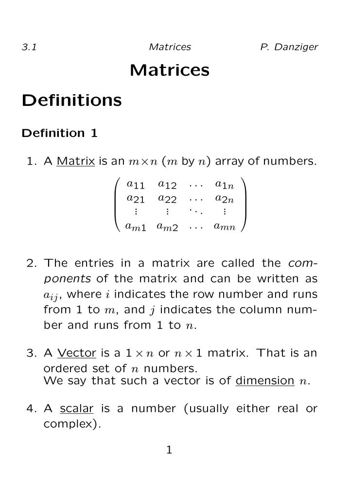
  1. 3.1 Matrices P. Danziger Matrices Definitions Definition 1 1. A Matrix is an m × n ( m by n ) array of numbers.   a 11 a 12 . . . a 1 n a 21 a 22 . . . a 2 n   . . .  ...  . . . . . .     a m 1 a m 2 . . . a mn 2. The entries in a matrix are called the com- ponents of the matrix and can be written as a ij , where i indicates the row number and runs from 1 to m , and j indicates the column num- ber and runs from 1 to n . 3. A Vector is a 1 × n or n × 1 matrix. That is an ordered set of n numbers. We say that such a vector is of dimension n . 4. A scalar is a number (usually either real or complex). 1
  2. 3.1 Matrices P. Danziger Notation 2 • We generally use uppercase letters from the beginning of the alphabet ( A, B, C . . . ) to de- note matrices. • A matrix is identified with its components, given a matrix A with components a ij , 1 ≤ i ≤ m , 1 ≤ j ≤ n , we may write A = [ a ij ] Example 3 Find the 4 × 4 matrix A with compoents given by a ij = i + j .  1 2 3 4  2 3 4 5     3 4 5 6     4 5 6 7 2

  3. 3.1 Matrices P. Danziger • We generally use lowercase boldface letters from the end of the alphabet ( u , v , w . . . ) to denote vectors. • We use the convention that u = ( u 1 , u 2 , . . . , u n ), x = ( x 1 , x 2 , . . . , x n ), etc. • If x = ( x 1 , x 2 , . . . , x n ) then the scalars x 1 , x 2 , . . . , x n are called the components of x . • We denote the set of all vectors of dimension n whose components are real numbers by R n . • We denote the set of all vectors of dimension n whose components are complex numbers by C n . Note This definition of vector differs from the usual ‘High School’ definition involving magnitude and direction. 3

  4. 3.1 Matrices P. Danziger Special Matrices and Vectors 1. The Identity matrix The identity matrix is a square matrix with 1’s down the diagonal, and zeros elsewhere. The n × n identity matrix is denoted I n .  1 0 0  . . . 0 1 0 . . .   I n =  . . .  ... . . . . . .     0 0 1 . . . 2. The Zero Matrix The zero matrix is an m × n matrix, all of whose entries are 0.  0 0 0  . . . 0 0 0 . . .    . . .  ... . . . . . .     0 0 0 . . . 4

  5. 3.1 Matrices P. Danziger Operations on Matrices 1. Transpose Given an m × n matrix, A , the transpose of A is obtained by interchanging the rows and columns of A . We denote the transpose of A by A t , or A T . Notes: • If A is m × n then A T will be n × m . • If A = [ a ij ], then [ a ij ] T = [ a ji ]. Example 4   1 4 � t (a) � 1 2 3 = 2 5   4 5 6   3 6 t     1 2 3 1 4 7 (b) 4 5 6 = 2 5 8         7 8 9 3 6 9   1 (c) (1 , 2 , 3) t = 2     3 5

  6. 3.1 Matrices P. Danziger 2. Matrix Addition Given two m × n matrices     a 11 a 12 . . . a 1 n b 11 b 12 . . . b 1 n a 21 a 22 . . . a 2 n b 21 b 22 . . . b 2 n     A = B =  ,  . . .   . . .  ... ... . . . . . . . . . . . .        a m 1 a m 2 . . . a mn b m 1 b m 2 . . . b mn We may define the sum of A and B , A + B , to be the sum componentwise, i.e.  a 11 + b 11 a 12 + b 12 a 1 n + b 1 n  . . . a 21 + b 21 a 22 + b 22 a 2 n + b 2 n . . .   A + B =  . . .  ... . . . . . .     a m 1 + b m 1 a m 2 + b m 2 a mn + b mn . . . � � � � � � Componentwise: + = a ij + b ij . a ij b ij This works for vectors as well. u + v = ( u 1 , u 2 , . . . , u n ) + ( v 1 , v 2 , . . . , v n ) = ( u 1 + v 1 , u 2 + v 2 , . . . , u n + v n ) Note that matrix addition is only defined if A and B have the same size. 6

  7. 3.1 Matrices P. Danziger Example 5 (a)     1 2 3 10 11 12 4 5 6  + 13 14 15        7 8 9 16 17 18   1 + 10 2 + 11 3 + 12 = 4 + 13 5 + 14 6 + 15     7 + 16 8 + 17 9 + 18   11 13 15 = 17 19 21     23 25 27 (b) (1 , 2 , 3) + (4 , 5 , 6) = (1 + 4 , 2 + 5 , 3 + 6) = (5 , 7 , 9) 7

  8. 3.1 Matrices P. Danziger 3. Matrix Multiplication (a) Scalar Multiplication Given a matrix A , and a scalar k , we de- fine the scalar product of k with A , kA by multiplying each entry of A by k .   a 11 a 12 . . . a 1 n a 21 a 22 . . . a 2 n   kA = k  . . .  ... . . . . . .     a m 1 a m 2 . . . a mn   ka 11 ka 12 . . . ka 1 n ka 21 ka 22 . . . ka 2 n   =  . . .  ... . . . . . .     ka m 1 ka m 2 . . . ka mn � � � � Componentwise: k = . a ij ka ij Note that this works for vectors as well. k u = k ( u 1 , u 2 , . . . , u n ) = ( ku 1 , ku 2 , . . . , ku n ) 8

  9. 3.1 Matrices P. Danziger Example 6     1 2 3 10 20 30 10 4 5 6  = 40 50 60        7 8 9 70 80 90 9

  10. 3.1 Matrices P. Danziger (b) Matrix Multiplication If A and B are two matrices where A has the same number of columns as B has rows (i.e. A is m × n and B is n × r ) we define the matrix product, AB to be the matrix in which the i, j th entry is made up of the dot product of the i th row of A with the j th column of B .   a 11 a 12 . . . a 1 n a 21 a 22 . . . a 2 n   A =  , . . . ... . . .   . . .  a m 1 a m 2 . . . a mn   b 11 b 12 . . . b 1 r b 21 b 22 . . . b 2 r   B = . . . ... . . .   . . .   b n 1 b n 2 . . . b nr     a 11 a 12 . . . a 1 n b 11 b 12 . . . b 1 r a 21 a 22 . . . a 2 n b 21 b 22 . . . b 2 r     AB = . . . . . . ... ... . . . . . .     . . . . . .     a m 1 a m 2 . . . a mn b n 1 b n 2 . . . b nr  a 11 b 11 + a 12 b 21 + . . . + a 1 n b n 1 a 11 b 1 r + a 12 b 2 r + . . . + a 1 n b . . . a 21 b 11 + a 22 b 21 + . . . + a 2 n b n 1 a 21 b 1 r + a 22 b 2 r + . . . + a 2 n b . . .  = . . ... . .  . .  a m 1 b 11 + a m 2 b 21 + . . . + a mn b n 1 a m 1 b 1 r + a m 2 b 2 r + . . . + a mn . . . 10

  11. 3.1 Matrices P. Danziger Example 7     1 2 3 9 8 7  = 4 5 6 6 5 4    7 8 9 3 2 1   1 × 9 + 2 × 6 + 3 × 3 1 × 8 + 2 × 5 + 3 × 2 1 × 7 + 2 × 4 + 3 × 1 4 × 9 + 5 × 6 + 6 × 3 4 × 8 + 5 × 5 + 6 × 2 4 × 7 + 5 × 4 + 6 × 1   7 × 9 + 8 × 6 + 9 × 3 7 × 8 + 8 × 5 + 9 × 2 7 × 7 + 8 × 4 + 9 × 1   9 + 12 + 9 8 + 10 + 6 7 + 8 + 3 = 36 + 30 + 18 32 + 25 + 12 28 + 20 + 6   63 + 48 + 27 56 + 40 + 18 49 + 32 + 9   30 24 18 = 84 69 54   138 114 90 Note that Matrix multiplication is only de- fined if A has the same number of columns as B has rows. 11

  12. 3.1 Matrices P. Danziger BIG Note Matrix multiplication is NOT commutative. i.e. It is NOT true that AB = BA (where defined). Example 8 � � � � � � 0 1 0 2 1 0 = 1 0 1 0 0 2 � � � � � � 0 2 0 1 2 0 = 1 0 1 0 0 1 12

Download Presentation
Download Policy: The content available on the website is offered to you 'AS IS' for your personal information and use only. It cannot be commercialized, licensed, or distributed on other websites without prior consent from the author. To download a presentation, simply click this link. If you encounter any difficulties during the download process, it's possible that the publisher has removed the file from their server.

Recommend


More recommend