Mathematical Analysis and Computational Simulations for flows of - - PowerPoint PPT Presentation

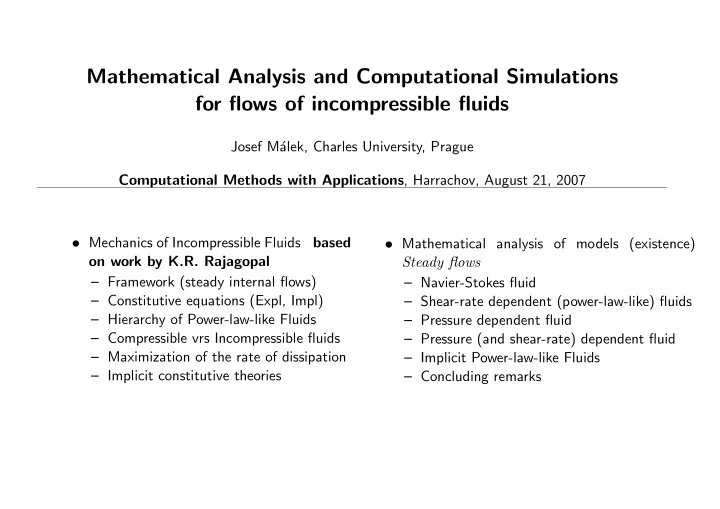
Mathematical Analysis and Computational Simulations for flows of incompressible fluids

Josef M´ alek, Charles University, Prague Computational Methods with Applications, Harrachov, August 21, 2007

• Mechanics of Incompressible Fluids

based

• n work by K.R. Rajagopal

– Framework (steady internal flows) – Constitutive equations (Expl, Impl) – Hierarchy of Power-law-like Fluids – Compressible vrs Incompressible fluids – Maximization of the rate of dissipation – Implicit constitutive theories

• Mathematical analysis of models (existence)

Steady flows – Navier-Stokes fluid – Shear-rate dependent (power-law-like) fluids – Pressure dependent fluid – Pressure (and shear-rate) dependent fluid – Implicit Power-law-like Fluids – Concluding remarks

1

Incompressible Fluid Mechanics: Basic Framework/1

Goal: To describe flows of various fluid-like-materials exhibiting so different and so fascinating phenomena yet share one common feature: these materials are well approximated as incompressible. SubGoal: To understand theoretical foundations and mathematical properties of these models. ̺t + div ̺v = 0 (̺v)t + div(̺v ⊗ v) = div T + ̺f T · D − ρdψ dt = ξ with ξ ≥ 0

• ̺ density
• ψ Helmholtz free energy
• T · D stress power
• ξ rate of dissipation
• v = (v1, v2, v3) velocity
• f = (f1, f2, f3) external body forces
• T = (Tij)3

i,j=1 Cauchy stress

• D := D(v) := 1/2(∇v + (∇v)T)
• Homogeneous fluids (the density is constant) =

⇒ div v = tr D = 0 p := 1 3 tr T pressure

2

Incompressible Fluid Mechanics: Basic Framework/2

Steady flows in Ω ⊂ R3 (time discretizations lead to similar problems) div v = 0 div(v ⊗ v) − div S = −∇p + f in Ω v = 0

• n ∂Ω

T · D = ξ with ξ ≥ 0 Constitutive equations: Relation between the Cauchy stress T , of the form T = −pI + S, and the symmetric part of the velocity gradient D := D(v) g(T , D) = 0 Power-law-like Rheology (broad, accessible)

• Explicit S = µ(. . . )D

– Navier-Stokes Fluids S = µ∗D – Power-law Fluids S = µ∗|D|r−2D – Power-law-like Fluids S = µ(|D|2)D – Fluids with shear-rate dpt viscosity – Fluids with the yield stress – Fluids with activation criteria

• Implicit

– Fluids with the yield stress (Bingham, Herschel-Bulkley) – Fluids with activation criteria – Implicit Power-law-like Fluids – Fluids with S = µ(p)D – Fluids with S = µ(p, |D|2)D

3

Framework is sufficiently robust to model behavior of various type of fluid-like materials. Models are frequently used in many areas of engineering and natural sciences: mechanics of colloids and suspensions, biological fluid mechanics (blood, synovial fluid), elastohydrodynamics, ice mechanics and glaciology, food processing

4

Fluids with shear-rate dependent viscosities

ν(|D|2)

If v = (u(x2), 0, 0), then |D(v)|2 = 1/2|u′|2 ... shear rate.

• ν(|D|2) = µ∗|D|r−2

1 < r < ∞

• power-law model
• ν(|D|2) ց as |D|2 ր
• shear-rate thinning fluid (r < 2)
• ν(|D|2) = µ∗

0 + µ∗ 1|D|r−2

r > 2

• Ladyzhenskaya model (65)
• (Smagorinskii turbulence model: r = 3)

5

Fluids with the yield stress or the activation criteria/discontinuous stresses

• threshold value for the stress to start flow
• Bingham fluid
• Herschel-Bingham fluid
• drastic changes of the properties when certain

criterion is met

• formation and dissolution of blood
• chemical reactions/time scale

6

Discontinuous stresses described by a maximal monotone graph

T1 T2 T

Tmax shear rate shear rate T12

7

Implicit power-law-like fluids

• S

K=|u’(r)|

8

Fluids with pressure-dependent viscosities

ν(p)

ν(p) = exp(γp) Bridgman(31): ”The physics of high pressure” Cutler, McMickle, Webb and Schiessler(58) Johnson, Cameron(67), Johnson, Greenwood(77), Johnson, Tewaarwerk(80) elastohydrodynamics: Szeri(98) synovial fluids No global existence result.

• Renardy(86), local, (ν(p)

p

→ 0 as p → ∞)

• Gazzola(97), Gazzola, Secchi(98): local, severe restrictions

9

Fluids with shear- and pressure-dependent viscosities

ν(p, |D|2)

ν(p, |D|2) = (η∞ + η0 − η∞ 1 + δ|D|2−r) exp(γ p) Davies and Li(94), Gwynllyw, Davies and Phillips(96) ν(p, |D|2) = c0 p |D| r = 1 Schaeffer(87) - instabilities in granular materials ν(p, |D|2) = (A + (1 + exp(α p))−q + |D|2)

r−2 2

α > 0, A > 0 1 ≤ r < 2 0 ≤ q ≤ 1 2α r − 1 2 − rA(2−r)/2 Q.: Is the dependence of the viscosity on the pressure admissible in continuum mechanics and thermodynamics?

10

Compressible vrs Incompressible

Compressible fluid

T = T (ρ, ∇v) = ⇒ T = T (ρ, D(v)) T = α0(ρ, ID, I ID, I I ID)I + α1(ρ, ID, I ID, I I ID)D + α2(ρ, ID, I ID, I I ID)D2 ID := tr D, I ID := 1 2

• [tr D]2 − tr D2
• ,

I I ID := det D Linearized model: T = ˆ α0(ρ)I + λ(ρ)[tr D]I + 2µ(ρ)D, Navier-Stokes fluid Usually: ˆ α0(ρ) is −p(ρ) thermodynamic pressure constitutive relation for p(ρ) needed to close the model = ⇒ λ, µ depends on pressure

Incompressible fluid

T = −pI + ˆ α1(I ID, I I ID)D + ˆ α2(I ID, I I ID)D2 Drawbacks:

• p in general is not the mean normal stress
• Can ˆ

αi depend on p? No, as the derivation based on the principle: Constraints do no work

11

Maximization of the rate of dissipation subject to two constraints

Assume ξ = 2 ν(tr T , |D|2)|D|2 and ψ = ψ(θ, ρ) = const Maximizing ξ with respect to D on the manifold described by the constraints (1) ξ = T · D (2) div v = tr D = 0 results to ∂ξ ∂D − λ1I − λ2(T − ∂ξ ∂D) = 0 = ⇒ T = −pI + 2 ν(p, |D|2)D with p := 1 3 tr T Viscosity: resistance between two sliding surfaces of fluids

12

Implicit theories

Derivation of the model from the implicit constitutive eqn g(T , D) = 0 Isotropy of the material implies α0I + α1T + α2D + α3T 2 + α4D2 + α5(T D + DT ) + α6(T 2D + DT 2) + α7(T D2 + D2T ) + α8(T 2D2 + D2T 2) = 0 αi being a functions of ρ, tr T , tr D, tr T 2, tr D2, tr T 3, tr D3, tr(T D), tr(T 2D), tr(D2T ), tr(D2T 2) For incompressible fluids T = 1 3 tr T I + ν(tr T , tr D2)D

13

Analysis of PDEs - Existence of (weak) solution - steady flows

• Mathematical consistency of the model (well-posedness), existence for any data in a reasonable

function space

• Notion of the solution: balance equations for any subset of Ω ⇐

⇒ weak solution ⇐ ⇒ FEM

• Choice of the function spaces
• To know what is the object we approximate
• Ω ⊂ R3 open, bounded with the Lipschitz boundary ∂Ω

div v = 0 − div(2ν(p, |D(v)|2)D(v)) + div(v ⊗ v) = −∇p + f in Ω (1) v = 0

• n ∂Ω

1 |Ω|

Ω

pdx = p0 (2) (0) ν(...) = ν0 NSEs (1) ν(...) = ν(|D|2) (2) ν(...) = ν(p, |D|2) (3) discontinuous (implicit) power-law fluids

14

NSEs

div v = 0 − µ∗∆v + div(v ⊗ v) = −∇p + f in Ω Step 1. Finite-dimensional approximations: (vN, pN) - Fixed-point iterations Step 2. Uniform estimates: supN ∇vN)2

2 + supN pN2 2 ≤ K

Step 3. Weak compactness: ∇vN → v and pN → p weakly in L2 Step 4. Nonlinearity tretaed by compact embedding: vN → v strongly in L2 Step 5. Limit in approximations as N → ∞ µ∗(∇vN, ∇ϕ) − (vN ⊗ vN, ∇ϕ) = (pN, div ϕ) + f, ϕ ∀ϕ (v, p) is a solution

15

µ(|D(v)|2) = µ∗|D(v)|r−2D(v)

• Critical values for the power-law index

div v = 0 − µ∗ div(|D(v)|r−2D(v)) + div(v ⊗ v) = −∇p + f in Ω Energy estimates: supN ∇vNr

r ≤ K - expect that v ∈ W 1,r 0,div(Ω)

• Equation for the pressure: p = (−∆)−1 div div(v ⊗ v − µ∗|D(v)|r−2D(v))

W 1,r ֒ → L3r/(3−r) = ⇒ v ⊗ v ∈ L

3r 2(3−r) and |D(v)|r−2D(v) ∈ Lr′ with r′ := r/(r − 1)

r r − 1 ≤ 3r 2(3 − r) ⇐ ⇒ r ≥ 9 5

• If v, ϕ ∈ W 1,r then v ⊗ v · ∇ϕ ∈ L1 only for r ≥ 9

5

• For r ≥ 9

5 the energy equality holds, higher differentiability accessible (useful tools)

– Compactness of the quadratic nonlinearity requires W 1,r ֒ →֒ → L2: holds for r ≥ 6

5

Analysis easier for r ≥ 9/5 and more difficult for r ∈ (6/5, 9/5) , in both cases more difficult than NSEs

16

Results for µ(|D(v)|2) = µ∗|D(v)|r−2D(v)

Th1 (Ladyzhenskaya, Lions 1967) Let r ≥ 9/5 and f ∈

• W 1,r

(Ω)3

and p0 ∈ R (D) Then there is a weak solution (v, p) to (1)-(2) such that v ∈ W 1,r

0,div(Ω)

and p ∈ Lr′ (Ω) Tools: Monotone operator theory, Minty method (energy equality), compact embedding Th2 (Frehse, Malek, Steinhauer 2003 and Diening, Malek, Steinhauer 2006) Let r ∈ (6/5, 9/5) and (D) hold. Then there is a weak solution (v, p) to (1)-(2) such that v ∈ W 1,r

0,div(Ω)

and p ∈ L3r/(2(r−1))(Ω) Tools: Lipschitz approximations of Sobolev functions (strengthened version), Strictly monotone

• perator, Minty method, compact embedding

17

Assumptions on µ’s for µ(p, |D(v)|2)

(A1) given

r ∈ (1, 2) there are C1 > 0 and C2 > 0 such that for all symmetric matrices B, D and all p C1(1 + |D|2)

r−2 2 |B|2 ≤

∂

(µ(p, |D|2)D

∂D · (B ⊗ B) ≤ C2(1 + |D|2)

r−2 2 |B|2

(A2) for all symmetric matrices D and all p

• ∂[µ(p, |D|2)D]

∂p

• ≤ γ0(1 + |D|2)

r−2 4

≤ γ0 γ0 < 1 Cdiv,2 C1 C1 + C2 .

The constant Cdiv,q occurs in the problem: For a given g ∈ Lq(Ω) with zero mean value to find z ∈ W 1,q (Ω) solving div z = g in Ω, z = 0 on ∂Ω and z1,q ≤ Cdiv,qgq. (3) The solvability: Bogovskij (79) or Amrouche, Girault (94).

18

Results for µ(p, |D(v)|2)

Th3 (Franta, Malek, Rajagopal 2005) Let r ∈ (9/5, 2) and (D) hold. Assume that (A1)–(A2) are fullfiled. Then there is a weak solution (v, p) to (1)-(2) such that v ∈ W 1,r

0,div(Ω)

and p ∈ Lr′ (Ω) Tools: Quasicompressible approximations, structure of the viscosities, solvability of equation div z = g, strictly monotone operator theory in D-variable, compactness for the velocity gradient, compactness for the pressure, compact embedding Th4 (Bul´ ıcek, Fiˇ serov´ a 2007) Let r ∈ (6/5, 9/5) and (D) holds. Assume that (A1)–(A2) are

• fullfiled. Then there is a weak solution (v, p) to (1)-(2) such that

v ∈ W 1,r

0,div(Ω)

and p ∈ L3r/(2(r−1))(Ω) Tools: Quasicompressible approximations, Lipschitz approximations of Sobolev functions (strengthened version), structure of the viscosities, solvability of equation div z = g, strictly monotone

• perator theory in D-variable, compactness for the velocity gradient, compactness for the pressure,

decomposition of the pressure, compact embedding

19

Implicit Power-Law-like Fluids

Power-law index r ∈ (1, ∞), its dual r′ := r/(r − 1) v ∈ W 1,r

0,div(Ω), S ∈ Lr′(Ω)3×3, , p ∈ L˜ r(Ω) with ˜

r = min{r′,

3r 2(3−r)}

div (v ⊗ v + pI − S) = f in D′(Ω), (Dv(x), S(x)) ∈ A(x) for all x ∈ Ωa.e. (4)

20

Properties of the maximal monotone graph A a.e.

(B1) (0, 0) ∈ A(x); (B2) If (D, S) ∈ R3×3

sym × R3×3 sym fulfils

(¯ S − S) · ( ¯ D − D) ≥ 0 for all ( ¯ D, ¯ S) ∈ A(x), then (D, S) ∈ A(x) (A is maximal monotone graph); (B3) There are a non-negative m ∈ L1(Ω) and c > 0 such that for all (D, S) ∈ A(x) S · D ≥ −m(x) + c(|D|r + |S|r′ ) (A is r − graph); (5) (B4) At least one of the following two conditions (I) and (II) happens: (I) for all (D1, S1) and (D2, S2) ∈ A(x) fulfilling D1 = D2 we have (S1 − S2) · (D1 − D2) > 0, (II) for all (D1, S1) and (D2, S2) ∈ A(x) fulfilling S1 = S2 we have (S1 − S2) · (D1 − D2) > 0,

21

Results for Implicit Power-law-like Fluids

Th5 (Malek, Ruzicka, Shelukhin 2005) Let r ∈ (9/5, 2) and (D) hold. Consider Herschel-Bulkley

• fluids. Then there is a weak solution (v, p, S) to (4).

Tools: Local regularity method free of involving the pressure, higher-differentiability, uniform monotone

• perator properties, compact embedding

Th6 (Gwiazda, Malek, Swierczewska 2007) Let r ≥ 9/5 and (D) holds. Assume that (B1)–(B4) are fullfiled. Then there is a weak solution (v, p, S) satisfying (4). Tools: Young measures (generalized version), energy equality, strictly monotone operator, compact embedding Th7 (Gwiazda, Malek, Swierczewska 2007) Let r > 6/5 and (D) holds. Assume that (B1)–(B4) are fullfiled. Then there is a weak solution (v, p, S) satisfying (4). Tools: Characterizatition of maximal monotone graphs in terms of 1-Lipschitz continuous mappings (Francfort, Murat, Tartar), Young measures, biting lemma, Lipschitz approximations of Sobolev functions (strengthened version), approximations of discontinuous functions, compact embedding

22

Concluding Remarks

• Consistent thermomechanical basis for incompressible fluids with power-law-like rheology
• ’Complete’ set of results concerning mathematical analysis of these models (sophisticated methods,

new tools)

• Computational tests (will be presented by M. M´

adl´ ık, J. Hron, M. Lanzend¨

• rfer) require numerical

analysis of the models

• Hierarchy is incomplete 1: unsteady flows, full thermodynamical setting
• Hierarchy is incomplete 2: rate type fluid models
• Mutual interactions (includes more realistic boundary conditions - I/O)

23

• 1. J. M´

alek and K.R. Rajagopal: Mathematical Issues Concerning the Navier-Stokes Equations and Some of Its Generalizations, in: Handbook of Differential Equations, Evolutionary Equations, volume 2 371-459 2005

• 2. J. Frehse, J. M´

alek and M. Steinhauer: On analysis of steady flows of fluids with shear-dependent viscosity based on the Lipschitz truncation method, SIAM J. Math. Anal. 34, 1064-1083, 2003

• 3. L. Diening, J. M´

alek and M. Steinhauer: On Lipschitz truncations of Sobolev functions (with variable exponent) and their selected applications, accepted to ESAIM: COCV, 2006

• 4. J. Hron, J. M´

alek and K.R. Rajagopal: Simple Flows of Fluids with Pressure Dependent Viscosities,

• Proc. London Royal Soc.: Math. Phys. Engnr. Sci. 457, 1603–1622, 2001
• 5. M. Franta, J. M´

alek and K.R. Rajagopal: Existence of Weak Solutions for the Dirichlet Problem for the Steady Flows of Fluids with Shear Dependent Viscosities, Proc. London Royal Soc. A:

• Math. Phys. Engnr. Sci. 461, 651–670 2005
• 6. J. M´

alek, M. R˚ uˇ ziˇ cka and V.V. Shelukhin: Herschel-Bulkley Fluids: Existence and regularity of steady flows, Mathematical Models and Methods in Applied Sciences, 15, 1845–1861, 2005

• 7. P. Gwiazda, J. M´

alek and A. ´ Swierczewska: On flows of an incompressible fluid with a discontinuous power-law-like rheology, Computers & Mathematics with Applications, 53, 531–546, 2007

• 8. M. Bul´

ıˇ cek, P. Gwiazda, J. M´ alek and A. ´ Swierczewska-Gwiazda: On steady flows of an incompressible fluids with implicit power-law-like theology, to be submitted 2007