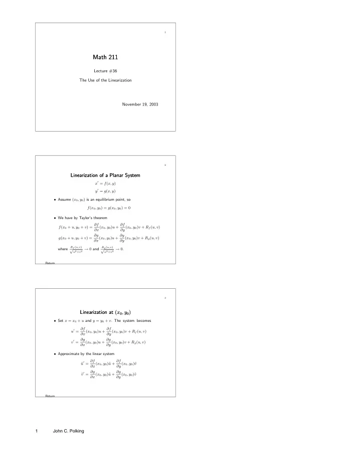
Math 211 Math 211 Lecture #36 The Use of the Linearization - - PDF document

1

Math 211 Math 211

Lecture #36 The Use of the Linearization November 19, 2003

Return

2

Linearization of a Planar System Linearization of a Planar System

x′ = f(x, y) y′ = g(x, y)

• Assume (x0, y0) is an equilibrium point, so

f(x0, y0) = g(x0, y0) = 0

• We have by Taylor’s theorem

f(x0 + u, y0 + v) = ∂f ∂x(x0, y0)u + ∂f ∂y (x0, y0)v + Rf(u, v) g(x0 + u, y0 + v) = ∂g ∂x(x0, y0)u + ∂g ∂y (x0, y0)v + Rg(u, v) where

Rf (u,v)

√

u2+v2 → 0 and Rg(u,v)

√

u2+v2 → 0.

Return

3

Linearization at (x0, y0) Linearization at (x0, y0)

• Set x = x0 + u and y = y0 + v. The system becomes

u′ = ∂f ∂x(x0, y0)u + ∂f ∂y (x0, y0)v + Rf(u, v) v′ = ∂g ∂x(x0, y0)u + ∂g ∂y (x0, y0)v + Rg(u, v)

• Approximate by the linear system

˜ u′ = ∂f ∂x(x0, y0)˜ u + ∂f ∂y (x0, y0)˜ v ˜ v′ = ∂g ∂x(x0, y0)˜ u + ∂g ∂y (x0, y0)˜ v

1 John C. Polking

Return Original system

4

Matrix Form of the Linearization Matrix Form of the Linearization

• Set u = (˜

u, ˜ v)T and introduce the Jacobian matrix J =

 

∂f ∂x(x0, y0) ∂f ∂y (x0, y0) ∂g ∂x(x0, y0) ∂g ∂y (x0, y0)

 

The linearization becomes u′ = Ju.

• We can solve the linear system explicitly.
• The linearization gives us information about the original

system.

Return Matrix form

5

Theorem 1 Theorem 1

Theorem: Consider the planar system x′ = f(x, y) y′ = g(x, y) where f and g are continuously differentiable. Suppose that (x0, y0) is an equilibrium point. If the linearization at (x0, y0) has a generic equilibrium point at the origin, then the equilibrium point at (x0, y0) is of the same type.

• Generic types: Saddle, nodal source, nodal sink, spiral

source, and spiral sink. — All occupy large open subsets of the trace-determinant plane.

• Nongeneric types: Center and others. — Occupy pieces of

the boundaries between the generic points.

Return Theorem

6

Examples Examples

• Center.

x′ = y + αx(x2 + y2) y′ = −x + αy(x2 + y2)

α > 0 ⇒ (0, 0)T is unstable. α < 0 ⇒ (0, 0)T is a sink.

• Competing species.

x′ = (5 − 2x − y)x y′ = (7 − 2x − 3y)y

• Default system in pplane.

2 John C. Polking

Return

7

Linear Analysis of Equilibrium Points Linear Analysis of Equilibrium Points

• Provides a good qualitative picture of how solutions behave

near generic equilibrium points.

• Provides limited qualitative information about the solutions

near nongeneric equilibrium points.

A linear center could be a spiral source or a spiral sink.

• Provides no information about the global behavior of

solutions to nonlinear systems.

Return Planar system Planar linearization

8

Higher Dimensional Systems Higher Dimensional Systems

Autonomous equation y′ = f(y).

• y = (y1, y2, · · · , yn)T , y0 is an equilibrium point.
• f(y) = (f1(y), f2(y), · · · , fn(y))T
• J is the Jacobian matrix
• f(y0 + u) = J(y0)u + R(u) where limu→0 R(u)

|u|

= 0.

• Set y = y0 + u. The system becomes

u′ = J(y0)u + R(u).

• The linearization is u′ = J(y0)u.

Return Linearization Theorem 1

9

Theorem 2 Theorem 2

Theorem: Suppose that y0 is an equilibrium point for y′ = f(y). Let J be the Jacobian of f at y0.

• 1. Suppose that the real part of every eigenvalue of J is
• negative. Then y0 is an asymptotically stable equilibrium

point.

• 2. Suppose that J has at least one eigenvalue with positive

real part. Then y0 is an unstable equilibrium point.

3 John C. Polking

Return Linear analysis

10

Example Example

x′ = −2x − 4y + 2xy y′ = x − 6y + x2 − y2

• The origin (0, 0) is an equilibrium point.
• The Jacobian has one eigenvalue, λ = −4, of algebraic

multiplicity 2.

• First theorem does not apply.
• Second theorem ⇒ the origin is a sink.

11

The Lorenz System The Lorenz System

x′ = −ax + ay y′ = rx − y − xz z′ = −bz + xy

• Use a = 10, b = 8/3, and r = 5, 20, 28, 100.

4 John C. Polking