Math 211 Math 211 Lecture #19 November 2, 2000 2 Planar System x - PDF document

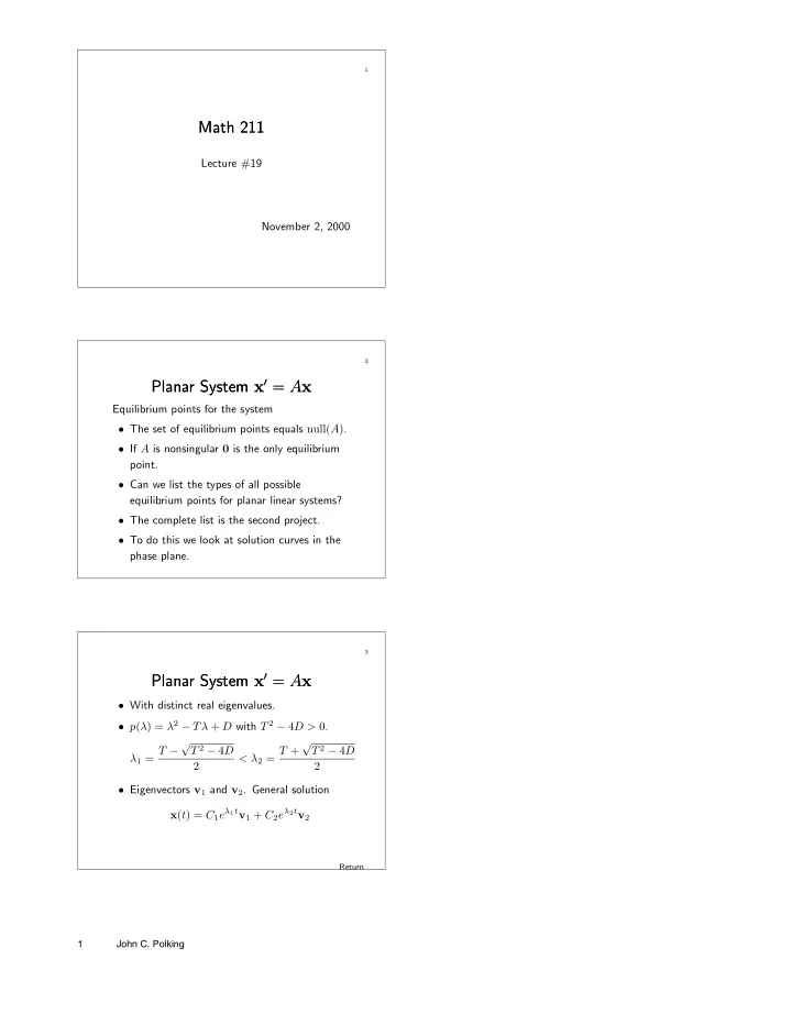
1 Math 211 Math 211 Lecture #19 November 2, 2000 2 Planar System x ′ = A x Planar System x ′ = A x Equilibrium points for the system • The set of equilibrium points equals null( A ) . • If A is nonsingular 0 is the only equilibrium point. • Can we list the types of all possible equilibrium points for planar linear systems? • The complete list is the second project. • To do this we look at solution curves in the phase plane. 3 Planar System x ′ = A x Planar System x ′ = A x • With distinct real eigenvalues. • p ( λ ) = λ 2 − Tλ + D with T 2 − 4 D > 0 . √ √ T 2 − 4 D T 2 − 4 D λ 1 = T − < λ 2 = T + 2 2 • Eigenvectors v 1 and v 2 . General solution x ( t ) = C 1 e λ 1 t v 1 + C 2 e λ 2 t v 2 Return 1 John C. Polking

4 Exponential Solutions Exponential Solutions x ( t ) = Ce λt v • The solution curve is a straight half-line through C v . • If λ > 0 the solution starts at 0 for t = −∞ , and tends to ∞ as t → ∞ . Unstable solution • If λ < 0 the solution starts at ∞ for t = −∞ , and tends to 0 as t → ∞ . Stable solution • Sometimes called half-line solutions. Real eigenvalues 5 Saddle Point Saddle Point • λ 1 < 0 < λ 2 • General solution x ( t ) = C 1 e λ 1 t v 1 + C 2 e λ 2 t v 2 • Two stable exponential solutions ( C 2 = 0 ) and two unstable exponential solutions ( C 1 = 0 ). • As t → ∞ , x ( t ) → ∞ approaching the half line through C 2 v 2 . • As t → −∞ , x ( t ) → ∞ approaching the half line through C 1 v 1 . 6 Nodal Sink Nodal Sink • λ 1 < λ 2 < 0 • General solution x ( t ) = C 1 e λ 1 t v 1 + C 2 e λ 2 t v 2 • Stable exponential solutions. • All solutions → 0 as t → ∞ . If C 2 � = 0 tangent to C 2 v 2 . All solutions are stable. • All solutions → ∞ as t → −∞ . If C 1 � = 0 parallel to the half line through C 1 v 1 . 2 John C. Polking

7 Nodal Source Nodal Source • 0 < λ 1 < λ 2 • General solution x ( t ) = C 1 e λ 1 t v 1 + C 2 e λ 2 t v 2 • Exponential solutions are unstable. • All solutions → 0 as t → −∞ . If C 1 � = 0 tangent to C 1 v 1 . All solutions are unstable. • All solutions → ∞ as t → −∞ . If C 2 � = 0 parallel to the half line through C 2 v 2 . 8 Planar System x ′ = A x Planar System x ′ = A x • Complex eigenvalues , λ = α + iβ and λ = α − iβ . ( T 2 − 4 D < 0 ) • Eigenvector w = v 1 + i v 2 associated to λ . • General real solution x ( t ) = C 1 e αt [cos βt · v 1 − sin βt · v 2 ] + C 2 e αt [sin βt · v 1 + cos βt · v 2 ] Return 9 Center Center • α = Re( λ ) = 0 • General real solution x ( t ) = C 1 [cos βt · v 1 − sin βt · v 2 ] + C 2 [sin βt · v 1 + cos βt · v 2 ] • Every solution is periodic with period T = 2 π/β. • All solution curves are ellipses. Complex eigenvalues Return 3 John C. Polking

10 Spiral Sink Spiral Sink • α = Re( λ ) < 0 • General real solution x ( t ) = C 1 e αt [cos βt · v 1 − sin βt · v 2 ] + C 2 e αt [sin βt · v 1 + cos βt · v 2 ] • All solutions spiral into 0 as t → ∞ . Complex eigenvalues Center 11 Spiral Source Spiral Source • α = Re( λ ) > 0 • General real solution x ( t ) = C 1 e αt [cos βt · v 1 − sin βt · v 2 ] + C 2 e αt [sin βt · v 1 + cos βt · v 2 ] • All solutions spiral into 0 as t → −∞ . Complex eigenvalues Center 12 Trace-Determinant Plane Trace-Determinant Plane � a 11 a 12 � p ( λ ) = λ 2 − Tλ + D A = ; a 21 a 22 √ T 2 − 4 D • Eigenvalues λ 1 , λ 2 = T ± . 2 p ( λ ) = ( λ − λ 1 )( λ − λ 2 ) = λ 2 − ( λ 1 + λ 2 ) λ + λ 1 λ 2 • T = λ 1 + λ 2 and D = λ 1 λ 2 . • Duality between ( λ 1 , λ 2 ) and ( T, D ) . Return 4 John C. Polking

13 Trace-Determinant Plane (cont.) Trace-Determinant Plane (cont.) • T 2 − 4 D > 0 ⇒ real eigenvalues λ 1 & λ 2 ⋄ D = λ 1 λ 2 < 0 ⇒ Saddle point. ⋄ D = λ 1 λ 2 > 0 ⇒ Eigenvalues have the same sign. ⋆ T = λ 1 + λ 2 > 0 Nodal source. ⋆ T = λ 1 + λ 2 < 0 Nodal sink. 14 Trace-Determinant Plane (cont.) Trace-Determinant Plane (cont.) • T 2 − 4 D < 0 ⇒ complex eigenvalues λ = α + iβ and λ = α − iβ. ⋄ T = λ + λ = 2 α > 0 ⇒ Spiral source ⋄ T = λ + λ = 2 α < 0 ⇒ Spiral sink ⋄ T = λ + λ = 2 α = 0 ⇒ Center 15 Generic and Nongeneric Generic and Nongeneric Equilibrium Points Equilibrium Points • Generic types ⋄ Saddle, nodal source, nodal sink, spiral source, and spiral sink. ⋄ All occupy large open subsets of the trace-determinant plane. • Nongeneric types ⋄ Center and all others. Occupy pieces of the boundaries. 5 John C. Polking

16 Higher Dimensional Systems Higher Dimensional Systems x ′ = A x • A is an n × n real matrix. • If λ is an eigenvalue and v � = 0 is an associated eigenvector, then x ( t ) = e λt v is a solution. 17 Suppose that λ 1 , . . . , λ k are Proposition: distinct eigenvalues of A , and that v 1 , . . . , v k are associated nonzero eigenvectors. Then v 1 , . . . , v k are linearly independent. Return 18 Suppose the n × n real matrix A Theorem: has n distinct eigenvalues λ 1 , . . . , λ n , and that v 1 , . . . , v n are associated nonzero eigenvectors. Then the exponential solutions x i ( t ) = e λ i t v i , 1 ≤ i ≤ n form a fundamental system of solutions for the system x ′ = A x . • Example 17 − 30 − 8   A = 16 − 29 − 8   − 12 24 7 Return 6 John C. Polking