Math 211 Math 211 Lecture #12 Eulers Method September 24, 2001 2 - PDF document

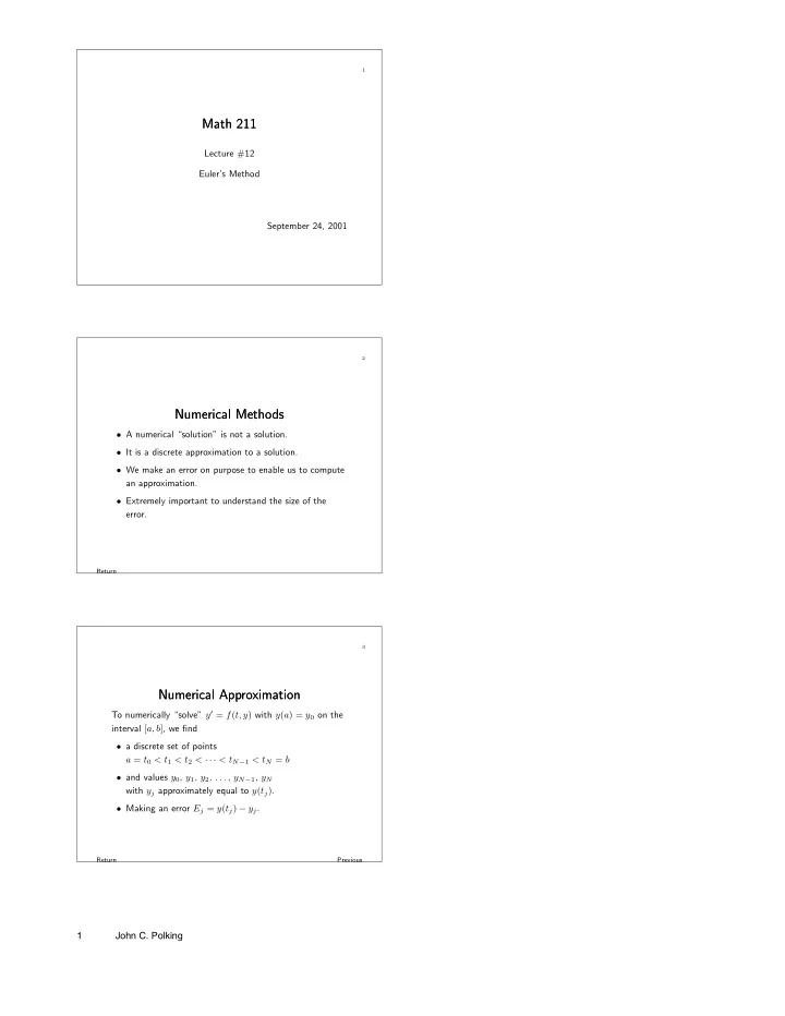
1 Math 211 Math 211 Lecture #12 Euler’s Method September 24, 2001 2 Numerical Methods Numerical Methods • A numerical “solution” is not a solution. • It is a discrete approximation to a solution. • We make an error on purpose to enable us to compute an approximation. • Extremely important to understand the size of the error. Return 3 Numerical Approximation Numerical Approximation To numerically “solve” y ′ = f ( t, y ) with y ( a ) = y 0 on the interval [ a, b ] , we find • a discrete set of points a = t 0 < t 1 < t 2 < · · · < t N − 1 < t N = b • and values y 0 , y 1 , y 2 , . . . , y N − 1 , y N with y j approximately equal to y ( t j ) . • Making an error E j = y ( t j ) − y j . Return Previous 1 John C. Polking

4 Types of Solvers Types of Solvers • We will discuss four solvers � Euler’s method, � second order Runge-Kutta, � fourth order Runge-Kutta, � and ode45 . • Everything works for first order systems almost without change. 5 Euler’s Method Euler’s Method • Solve (approximately) y ′ = f ( t, y ) with y ( a ) = y 0 on the interval [ a, b ] . • Discrete set of values of t . � t 0 = a , fixed step size h = ( b − a ) /N. � t 1 = t 0 + h , t 2 = t 1 + h = t 0 + 2 h , etc, � t N = a + Nh = b Return 6 Euler’s Method – First Step Euler’s Method – First Step • At each step approximate the solution curve by the tangent line. • First step: � y ( t 0 + h ) ≈ y ( t 0 ) + y ′ ( t 0 ) h. t 1 = t 0 + h � y ( t 1 ) ≈ y 0 + f ( t 0 , y 0 ) h. � Set y 1 = y 0 + f ( t 0 , y 0 ) h, so y ( t 1 ) ≈ y 1 . Return Numerical methods Time steps 2 John C. Polking

7 Euler’s Method – Second Step Euler’s Method – Second Step • At each step use the tangent line. • Second step – start at ( t 1 , y 1 ) . � New solution ˜ y with initial value ˜ y ( t 1 ) = y 1 . � ˜ y ( t ) ≈ ˜ y ( t 1 ) + ˜ y ′ ( t 1 )( t − t 1 ) , t 2 = t 1 + h � ˜ y ( t 2 ) ≈ y 1 + f ( t 1 , y 1 ) h. � Set y 2 = y 1 + f ( t 1 , y 1 ) h, so y ( t 2 ) ≈ ˜ y ( t 2 ) ≈ y 2 . Return Numerical methods Time steps 8 Euler’s Method – Algorithm Euler’s Method – Algorithm Input t 0 and y 0 . for k = 1 to N set y k = y k − 1 + f ( t k − 1 , y k − 1 ) h t k = t k − 1 + h Thus, y 1 = y 0 + f ( t 0 , y 0 ) h and t 1 = t 0 + h y 2 = y 1 + f ( t 1 , y 1 ) h and t 2 = t 1 + h y 3 = y 2 + f ( t 2 , y 2 ) h and t 3 = t 2 + h etc. Return Numerical methods Time steps 9 M ATLAB routine eulerdemo.m M ATLAB routine eulerdemo.m • Demonstrates truncation error. • Demonstrates how truncation error can propagate exponentially. • Demonstrates how the total error is the sum of propagated truncation errors. Return 3 John C. Polking

10 Error Analysis – First Step Error Analysis – First Step • Euler’s approximation y 1 = y 0 + f ( t 0 , y 0 ) h ; t 1 = t 0 + h • Taylor’s theorem y ( t 1 ) = y ( t 0 + h ) = y ( t 0 ) + y ′ ( t 0 ) h + R ( h ) | R ( h ) | ≤ Ch 2 • y ( t 1 ) − y 1 = R ( h ) Return 11 Error Analysis Error Analysis • The truncation error at each step is the same as the Taylor remainder, and | R ( h ) | ≤ Ch 2 . • There are N = ( b − a ) /h steps. Truncation error can grow exponentially. � e L ( b − a ) − 1 � Maximum error ≤ C h, where C & L are constants that depend on f . Return 12 Error Analysis Error Analysis � e L ( b − a ) − 1 � Maximum error ≤ C h, where C & L are constants that depend on f . • Good news: the error decreases as h decreases. • Bad news: the error can get exponentially large as the length of the interval [i.e., b-a] increases. Return 4 John C. Polking

13 M ATLAB routine eul.m M ATLAB routine eul.m Syntax: [t,y] = eul(derfile, [ t 0 , t f ] , y 0 , h ); • derfile - derivative m-file defining the equation. • t 0 - initial time; t f - final time. • y 0 - initial value. • h - step size. Return Algorithm 14 Derivative m-file Derivative m-file The derivative m-file describes the differential equation. • Example: y ′ = y 2 − t • Derivative m-file: function ypr = george(t,y) ypr = y^2 - t; • Save as george.m . Return 15 Use of eul.m Use of eul.m • Solve y ′ = y 2 − t . • Use the derivative m-file george.m . • Use t 0 = 0 , t f = 10 , y 0 = 0 . 5 , and several step sizes. • Syntax: [t,y] = eul( ′ george ′ ,[0,10],0.5,h); Return 5 John C. Polking

16 Experimental Error Analysis Experimental Error Analysis • IVP y ′ = cos( t ) / (2 y − 2) with y (0) = 3 • Exact solution: y ( t ) = 1 + √ 4 + sin t. • Solve using Euler’s method and compare with the exact solution. • Do this for several step sizes. Return Derivative m-file Batch file 17 Derivative m-file ben.m Derivative m-file ben.m function yprime = ben(t,y) yprime = cos(t)/(2*y-2); Experimental analysis Return 18 M-file batch.m M-file batch.m [teuler,yeuler]=eul(’ben’,[0,3],3,h); t=0:0.05:3; y=1+sqrt(4+sin(t)); plot(t,y,teuler,yeuler,’o’) legend(’Exact’,’Euler’) shg z=1+sqrt(4+sin(teuler)); maxerror=max(abs(z-yeuler)) Return Experimental analysis Good news 6 John C. Polking