Maps in Shape Collections Descriptor and Subspace Learning Feature - PowerPoint PPT Presentation

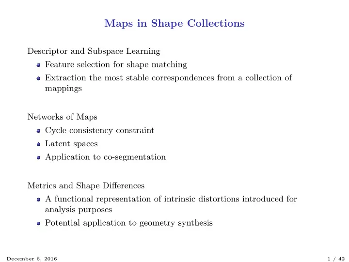
Maps in Shape Collections Descriptor and Subspace Learning Feature selection for shape matching Extraction the most stable correspondences from a collection of mappings Networks of Maps Cycle consistency constraint Latent spaces Application to co-segmentation Metrics and Shape Differences A functional representation of intrinsic distortions introduced for analysis purposes Potential application to geometry synthesis December 6, 2016 1 / 42

Part I Descriptor and Subspace Learning Feature selection for shape matching Extraction the most stable correspondences from a collection of mappings December 6, 2016 2 / 42

Functional Map Approximation Functional map approximation [Ovsjanikov et al., 2012]: � CA 0 − A i � 2 F + α � C∆ 0 − ∆ i C � 2 C ⋆ i = arg min F C M N A i functions on N i ∆ i Laplacian on N i December 6, 2016 3 / 42

Functional Map Approximation Functional map approximation [Ovsjanikov et al., 2012]: � CA 0 − A i � 2 F + α � C∆ 0 − ∆ i C � 2 C ⋆ i = arg min F C Probe functions Any functions stable by nearly-isometric deformation In practice: HKS [Sun et al., 2009], WKS [Aubry et al., 2011], Curvatures... ◮ Non-unique solution December 6, 2016 3 / 42

Functional Map Approximation Functional map approximation [Ovsjanikov et al., 2012]: � CA 0 − A i � 2 F + α � C∆ 0 − ∆ i C � 2 C ⋆ i = arg min F C Probe functions Any functions stable by nearly-isometric deformation In practice: HKS [Sun et al., 2009], WKS [Aubry et al., 2011], Curvatures... Regularization: Assume nearly isometric deformations Commutativity of C with the Laplace-Beltrami operator: C∆ 0 = ∆ i C ◮ It can be difficult to a obtain good approximation December 6, 2016 3 / 42

Main Challenges C ⋆ � CA 0 − A i � 2 F + α � C∆ 0 − ∆ i C � 2 i = arg min F C ◮ The probe functions can be inconsistent (a) Smoothed Gaussian curvature. (b) Logarithm of the absolute value of Gaussian Curvature. December 6, 2016 4 / 42

Main Challenges C ⋆ � CA 0 − A i � 2 F + α � C∆ 0 − ∆ i C � 2 i = arg min F C ◮ The probe functions can be inconsistent (a) Smoothed Gaussian curvature. (b) Logarithm of the absolute value of Gaussian Curvature. Weight the probe functions [Corman et al., 2014]: � CA 0 D − A i D � 2 F + α � C∆ 0 − ∆ i C � 2 C ⋆ i ( D ) = arg min F C December 6, 2016 4 / 42

Main Challenges C ⋆ � CA 0 − A i � 2 F + α � C∆ 0 − ∆ i C � 2 i = arg min F C ◮ The approximation is not reliable on the entire functional space C ⋆ f f December 6, 2016 5 / 42

Main Challenges C ⋆ � CA 0 − A i � 2 F + α � C∆ 0 − ∆ i C � 2 i = arg min F C ◮ The approximation is not reliable on the entire functional space C ⋆ f f Learn the functional subspace S p ⊂ L 2 ( M ) of dimension p such that: C T f ≈ C ⋆ f , ∀ f ∈ S p December 6, 2016 5 / 42

Feature Selection Training Set December 6, 2016 6 / 42

Feature Selection N N D ⋆ ∈ arg min � � � C ⋆ � ( C ⋆ i ( D ⋆ ) − C i ) Y � 2 i ( D ) − C i � ; Y p ∈ arg min F D Y ⊤ Y = I p i =1 i =1 Training Set C 1 C 2 C 3 C 4 C 5 December 6, 2016 6 / 42

Feature Selection N N D ⋆ ∈ arg min � � � C ⋆ � ( C ⋆ i ( D ⋆ ) − C i ) Y � 2 i ( D ) − C i � ; Y p ∈ arg min F D Y ⊤ Y = I p i =1 i =1 D ⋆ : optimal weights Training Set Y p : basis of S p C 1 C 2 C 3 C 4 C 5 December 6, 2016 6 / 42

Feature Selection N N D ⋆ ∈ arg min � � � C ⋆ � ( C ⋆ i ( D ⋆ ) − C i ) Y � 2 i ( D ) − C i � ; Y p ∈ arg min F D Y ⊤ Y = I p i =1 i =1 D ⋆ : optimal weights Training Set Y p : basis of S p Unseen shape C 1 C 2 C ⋆ p ( D ⋆ ) = C ( D ⋆ ) Y p C 3 C 4 C 5 December 6, 2016 6 / 42

Stable function subspace Reduced basis extraction: y 1 y 2 y 3 y 4 Correspondences: December 6, 2016 7 / 42

Non-Isometric matching Training Set Unseen Poses 100 basis functions 310 probe functions Training set: 10 shapes of women + 1 reference shape of man 50 functions in the reduced basis December 6, 2016 8 / 42

Results: Non Isometric matching December 6, 2016 9 / 42

Conclusion Naive Map Learned Map ◮ The functional maps quality can be improved by weighting the probe functions ◮ Learning makes the functional maps more stable with respect to large deformations December 6, 2016 10 / 42

Part II Network of Maps A non-supervised regularization for shape matching Cycle consistency constraint Latent spaces December 6, 2016 11 / 42

Graph of Maps 3 2 4 C 3 C 2 C 4 C 5 C 1 5 0 1 ◮ Compact description the entire network by composition (e.g. C 45 = C 05 C 40 ) December 6, 2016 12 / 42

Graph of Maps 3 2 4 C 3 C 2 C 4 C 5 C 1 5 0 1 ◮ Compact description the entire network by composition (e.g. C 45 = C 05 C 40 ) ◮ Suppose a star graph structure ◮ The results depends on the reference shape December 6, 2016 12 / 42

Graph of Maps 3 2 4 5 1 How to use general graph structure? How to impose coherence and consistency? How a shzpe collection help solving shape matching problem? December 6, 2016 13 / 42

Cycle Consistency Constraint Consistent Path December 6, 2016 14 / 42

Cycle Consistency Constraint Consistent Path Inconsistent Path December 6, 2016 14 / 42

Cycle Consistency Constraint Consistent Path Inconsistent Path ◮ Strong regularization ◮ Allows detection and correction of errors ◮ Characterized by: C ij = C kj C ik December 6, 2016 14 / 42

Cycle Consistency and Low Rank Matrix ◮ Can be difficult to enforce in an optimization problem: C ij = C kj C ik ◮ Equivalent to a low rank or semi-definiteness condition on a big mapping matrix [Huang et al., 2014]    Y +  C 11 · · · C N 1 1 . . . ... � � C := . .  = . · · · � 0     Y 1 Y N . . .    Y + C 1 N · · · C NN N December 6, 2016 15 / 42

Cycle Consistency and Low Rank Matrix ◮ Can be difficult to enforce in an optimization problem: C ij = C kj C ik ◮ Equivalent to a low rank or semi-definiteness condition on a big mapping matrix [Huang et al., 2014]    Y +  C 11 · · · C N 1 1 . . . ... � � C := . .  = . · · · � 0     Y 1 Y N . . .    Y + C 1 N · · · C NN N C is semi-definite Rank of C is very low compared to the number of shapes December 6, 2016 15 / 42

Computation of a Functional Map Network Given descriptors on each shape, we can compute the functional map network: C ⋆ = min � � C ij A i − A j � 2 , 1 + Reg( C ij ) + λ � C � ⋆ C ( i,j ) ∈G December 6, 2016 16 / 42

Computation of a Functional Map Network Given descriptors on each shape, we can compute the functional map network: C ⋆ = min � � C ij A i − A j � 2 , 1 + Reg( C ij ) + λ � C � ⋆ C ( i,j ) ∈G ◮ Nuclear norm � X � ⋆ = � i σ i ( X ) is the convex regularization of the rank ◮ Convex optimization problem solved with ADMM December 6, 2016 16 / 42

Computation of a Functional Map Network Given descriptors on each shape, we can compute the functional map network: C ⋆ = min � � C ij A i − A j � 2 , 1 + Reg( C ij ) + λ � C � ⋆ C ( i,j ) ∈G ◮ Nuclear norm � X � ⋆ = � i σ i ( X ) is the convex regularization of the rank ◮ Convex optimization problem solved with ADMM Unlike separate computation of the functional map this setting: ◮ Removes descriptors outliers ◮ Enforces coherence between in the network December 6, 2016 16 / 42

Latent Spaces 3 2 4 Y 3 Y 4 Y 2 ? Y 5 Y 1 5 1     Y + · · · C 11 C N 1 1 . . . ... � � . .  = . Y 1 · · · Y N     . . .    Y + · · · C 1 N C NN N December 6, 2016 17 / 42

Latent Spaces 3 2 4 Y 3 Y + 4 Y 5 Y 4 Y 2 ? Y 5 Y 1 5 1     Y + · · · C 11 C N 1 1 . . . ... � � . .  = . Y 1 · · · Y N     . . .    Y + · · · C 1 N C NN N December 6, 2016 17 / 42

Latent Spaces 3 2 4 Y 3 Y + 4 Y 5 Y 4 Y 2 ? Y 5 Y 1 5 1     Y + · · · C 11 C N 1 1 . . . ... � � . .  = . Y 1 · · · Y N     . . .    Y + · · · C 1 N C NN N ◮ The Y i can be understood as functional maps to an abstract surface called “latent space” December 6, 2016 17 / 42

Orthogonal Basis Synchronization Cycle consistency as hard constraint: � � C ij − Y + j Y i � 2 F s . t . Y ⊤ min i Y i = I Y 1 ,..., Y N ( i,j ) ∈G Given a map network C ij , ( i, j ) ∈ G (with possible inconsistencies and missing edges), performing the factorization can be used to: ◮ Regularize and clean up functional maps ◮ Extract shared structure ◮ Find the most representative reference abstract shape ◮ Efficient storage of large network December 6, 2016 18 / 42

Application to Cosegmentation [Huang et al., 2014] Input: Shape collection and local descriptors Output: Consistent segmentation ◮ Joint map optimization C ⋆ = min � � C ij A i − A j � 2 , 1 + λ � C � ⋆ C ( i,j ) ∈G December 6, 2016 19 / 42