macroscopic fluctuations in non equilibrium mean field
play

Macroscopic fluctuations in non-equilibrium mean-field diffusions - PowerPoint PPT Presentation

Macroscopic fluctuations in non-equilibrium mean-field diffusions Krzysztof Gaw edzki GGI, Florence, May 2014 Mean field approximation has served us for over 100 years ( Curie 1895, Weiss 1907) giving hints about the behavior of in high


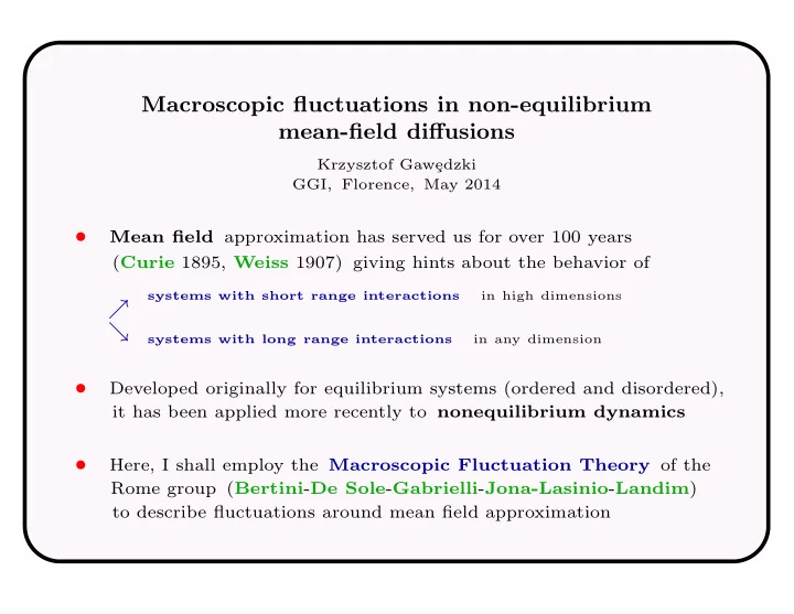
  1. Macroscopic fluctuations in non-equilibrium mean-field diffusions Krzysztof Gaw¸ edzki GGI, Florence, May 2014 • Mean field approximation has served us for over 100 years ( Curie 1895, Weiss 1907) giving hints about the behavior of in high dimensions systems with short range interactions ր ց systems with long range interactions in any dimension • Developed originally for equilibrium systems (ordered and disordered), it has been applied more recently to nonequilibrium dynamics • Here, I shall employ the Macroscopic Fluctuation Theory of the Rome group ( Bertini - De Sole - Gabrielli - Jona-Lasinio - Landim ) to describe fluctuations around mean field approximation
  2. • Informally, the Roman theory may be viewed as a version of Freidlin - Wentzell large deviations theory applied to stochastic lattice gases (zero range, SSEP, WASEP, ABC, ...) • We shall keep a similar point of view in application to general non-equilibrium d -dimensional diffusions with mean-field coupling: N � � dx n 1 = X ( t, x n ) + Y ( t, x n , x m ) + X a ( t, x n ) ◦ η na ( t ) dt N ր m =1 a independent white noises with Y ( x, y ) = − Y ( y, x ) and ◦ for the Stratonovich convention • Based on joint work with F. Bouchet and C. Nardini

  3. • Prototype model : N planar rotators with angles θ n and mean field coupling, undergoing Langevin dynamics N � � dθ n = F − H sin θ n − J sin( θ n − θ m ) + 2 k B T η n ( t ) dt N ր m =1 independent white noises Shinomoto - Kuramoto , Prog. Theor. Phys. 75 (1986), · · · · · · , Giacomin - Pakdaman - Pellegrin - Poquet , SIAM J. Math. Anal. 44 (2012) • Close cousin of the celebrated Kuramoto (1975) model for synchronization (with F → F n random and T = 0 ) whose versions were recently studied by the long-range community (papers by Gupta - Campa -( Dauxois )- Ruffo ) • Originally thought as a model of cooperative behavior of coupled nerve cells • Close to models of depinning transition in disordered elastic media

  4. • The Shinomoto - Kuramoto system N � � dθ n = F − H sin θ n − J sin( θ n − θ m ) + 2 k B T η n ( t ) dt N m =1 may also be re-interpreted as a classical ferromagnetic XY model � with a mean-field coupling of planar spins S n • F = 0 case ( equilibrium ) : � � � H = H, 0 in constant external magnetic field � � � S n = S cos θ n , sin θ n • F � = 0 case ( non-equilibrium ) : � � � H = H cos( F t ) , − sin( F t ) in rotating external magnetic field � � � ( i . e . spins are viewed in S n = S cos( θ n − F t ) , sin( θ n − F t ) frame ) the co − moving S S n n θ n H θ −Ft H n F = 0 F � = 0

  5. • Macroscopic quantities of interest in the general case N � � dx n 1 = X ( t, x n ) + Y ( t, x n , x m ) + X a ( t, x n ) ◦ η na ( t ) dt N m =1 a • empirical density N � 1 ρ N ( t, x ) = δ ( x − x n ( t )) N n =1 • empirical current N � 1 δ ( x − x n ( t )) ◦ dx n ( t ) j N ( t, x ) = N dt n =1 • They are related to each other by the continuity equation: ∂ t ρ N + ∇ · j N = 0 • Macroscopic Fluctuation Theory applies to their large deviations at N ≫ O (1) around N = ∞ mean field

  6. • Effective diffusion in the density space dxn ( t ) • Substitution of the equation of motion for and the passage dt to the Itˆ o convention give: N � j N ( t, x ) = 1 δ ( x − x n ( t )) ◦ dx n ( t ) = j ρN ( t, x ) + ζ ρN ( t, x ) N dt n =1 where � � � j ρ = ρ X + Y ∗ ρ − D ∇ ρ ← − ρ quadratic in with � � � � � X = X − 1 1 ∇ · X a X a , D = X a ⊗ X a 2 2 a a � ( Y ∗ ρ )( t, x ) ≡ Y ( t, x, y ) ρ ( t, y ) dy and N � � 1 � ζ ρN ( t, x ) = X a ( t, x ) δ x − x n ( t )) η na ( t ) N n =1 a

  7. • Conditioned w.r.t. ρ N , the noise ζ ρN ( t, x ) has the same law � 2 N − 1 D ( t, x ) ρ N ( t, x ) ξ ( t, x ) where as the white noise � � = δ ij δ ( t − s ) δ ( x − y ) ξ i ( t, x ) ξ j ( s, y ) • Follows from the fact that for functionals Φ[ ρ ] of (distributional) densities, the standard stochastic differential calculus gives � � � � � � d Φ[ ρ Nt ] = L Nt Φ [ ρ Nt ] dt where � � L Nt Φ � [ ρ ] = − δ Φ[ ρ ] δρ ( x ) ∇· j ρ ( t, x ) dx � � � δ 2 Φ[ ρ ] + 1 δρ ( x ) δρ ( y ) ∇ x ∇ y D ( t, x ) ρ ( t, x ) δ ( x − y ) dx dy N is the generator of the (formal) diffusion in the space of densities evolving according to the Itˆ o SDE � 2 N − 1 Dρ ξ � = 0 ∂ t ρ + ∇ · � j ρ +

  8. • N = ∞ closure • When N → ∞ , the evolution equation for the empirical density reduces to Nonlinear Fokker - Planck Equation ( NFPE ) � � � ˆ � ∂ t ρ = −∇ · j ρ = −∇ · ρ X + Y ∗ ρ − D ∇ ρ a nonlinear dynamical system in the space of densities → (autonomous or not) • If Y = 0 then the N = ∞ empirical density coincides with instantaneous PDF of identically distributed processes x n ( t ) and NFPE reduces to the linear Fokker - Planck equation for the latter • The N = ∞ phase diagram of an autonomous system with mean-field coupling is obtained by looking for stable stationary and periodic solutions of NFPE and their bifurcations • In principle, more complicated dynamical behaviors may also arise

  9. N = ∞ phases of the rotator model • • Stationary solutions of NFPE satisfy ∂ θ j ρ ( θ ) = 0 , i.e. � � � � 2 π � ∂ θ ρ ( θ ) F − H sin( θ ) − J sin( θ − ϑ ) ρ ( ϑ ) dϑ − k B T ∂ θ ρ ( θ ) 0 տ = sinθ cos ϑ − cos θ sin ϑ � � � � = ∂ θ ρ ( θ ) F − ( H + x 1 ) sin θ + x 2 cos θ − k B T ∂ θ ρ ( θ ) = 0 2 π � 2 π � with x 1 = J cos ϑ ρ ( ϑ ) dϑ , x 2 = J sin ϑ ρ ( ϑ ) 0 0 and the solution θ +2 π � F θ +( H + x 1) cos θ + x 2 sin θ − F ϑ +( H + x 1) cos ϑ + x 2 sin ϑ ρ ( θ ) = 1 kBT kB T Z e e dϑ θ • The coupled equations for 2 variables x 1 , x 2 may be easily analyzed

  10. • N = ∞ phase diagram for the rotator model for F � = 0 ( Shinomoto - Kuuramoto 1984, Sakaguchi - Shin .- Kur . 1986, ... ) Bogdanov H −Takens ordered H o e op d n e f l d d sa F periodic � � disordered �� �� � � � � � � �� �� � � � � �� �� � � � � � � � � �� �� �� �� � � � � �� �� � � � � � � � � �� �� 0 J 0.5 T k B • For H = 0 the periodic phase coincides with the ordered low-temp. equilibrium phase viewed in the co-rotating phase • When F ց 0 the periodic phase reduces to the equilibrium disordered phase at H = +0 • Global properties of the NFPE dynamics for the rotator model have been recently studied by Giacomin and collaborators

  11. • Fluctuations for N large but finite • Formally, domain of applications of the small-noise Freidlin - Wentzell large deviations theory • In Martin - Rose - Siggia formalism, the joint PDF of empirical density and current profiles is � �� � �� � � � � � � δ ρ − ρ N δ j − j N = δ ∂ t ρ + ∇ · j δ j − j ρ − ζ ρ � � � � � � a · ( j − jρ − ζρ ) D a e iN = δ ∂ t ρ + ∇ · j � � � � � a · ρD a D a e iN a · ( j − jρ ) − N = δ ∂ t ρ + ∇ · j � � � e − 1 ( j − jρ )( ρD ) − 1( j − jρ ) ∼ e − N I [ ρ,j ] 4 N ∼ δ ∂ t ρ + ∇ · j where the rate function(al) � � ( j − j ρ )( ρD ) − 1 ( j − j ρ ) dtdx 1 if ∂ t ρ + ∇ · j = 0 4 I [ ρ, j ] = ∞ otherwise

  12. • Large-deviations rate function(al)s for empirical densities or empirical currents only � � � � N →∞ e − N I [ ρ ] N →∞ e − N I [ j ] δ [ ̺ − ρ N ] ∼ δ [ j − j N ] ∼ are obtained by the contraction principle � � � ( −∇ · ρD ∇ ) − 1 � � 1 I [ ρ ] = min I [ ρ, j ] = ∂ t ρ + ∇· j ρ ∂ t ρ + ∇· j ρ dtdx 4 j I [ j ] = min I [ ρ, j ] with appropriate boundary limiting conditions for ρ ρ • That empirical densities have dynamical large deviations with rate function given above was proven by Dawson - Gartner in 1987 • To our knowledge, the large deviations of currents for mean field models were not studied in math literature • The formulae above have similar form as for the macroscopic density and current rate functions in stochastic lattice gases studied by the Rome group and B. Derrida with collaborators

  13. • Elements of the (Roman) Macroscopic Fluctuation Theory • Instantaneous fluctuations of empirical densities • Time t distribution of the empirical density � � ∼ e − N F t [ ̺ ] leading ← P t [ ̺ ] = δ [ ̺ − ρ Nt ] WKB term ∂ t P t = L † satisfies the functional equation Nt P t which reduces for the large-deviations rate function F t [ ̺ ] to the functional Hamilton - Jacobi Equation ( HJE ) � � � � � � j ρ · ∇ δ F t [ ̺ ] ∇ δ F t [ ̺ ] ∇ δ F t [ ̺ ] ∂ t F t [ ̺ ] + + · ρD = 0 δ̺ δ̺ δ̺ • In a stationary state the latter becomes the time-independent HJE for the rate function F [ ̺ ]

Download Presentation
Download Policy: The content available on the website is offered to you 'AS IS' for your personal information and use only. It cannot be commercialized, licensed, or distributed on other websites without prior consent from the author. To download a presentation, simply click this link. If you encounter any difficulties during the download process, it's possible that the publisher has removed the file from their server.

Recommend


More recommend