Machine Learning for Computational Linguistics Some probability - - PDF document

SLIDE 1

Machine Learning for Computational Linguistics

A refresher on probability and information theory Çağrı Çöltekin

University of Tübingen Seminar für Sprachwissenschaft

April 19/21, 2016

Probability theory Some probability distributions Information theory

Why probability theory?

▶ Probability theory studies uncertainty ▶ In machine learning we deal with problems with uncertainty,

because of

▶ inherently stochasticity of some physical systems ▶ incomplete/inaccurate measurements ▶ incomplete modeling Ç. Çöltekin, SfS / University of Tübingen April 19/21, 2016 1 / 48 Probability theory Some probability distributions Information theory

What is probability?

▶ Probability is a measure of (un)certainty of an event ▶ We quantify the probability of an event with a number

between 0 and 1

0 the event is impossible 0.5 the event is as likely to happen (or happened) as it is not 1 the event is certain

▶ All possible outcomes of an trial (experiment or observation)

is called the sample space (Ω) Axioms of probability states that

• 1. P(E) ∈ R, P(E) ⩾ 0
• 2. P(Ω) = 1
• 3. For disjoint events E1 and E2, P(E1 ∪ E2) = P(E1) + P(E2)

Ç. Çöltekin, SfS / University of Tübingen April 19/21, 2016 2 / 48 Probability theory Some probability distributions Information theory

Where do probabilities come from

Axioms of probability does not specify how to assign probabilities to events. Two major (rival) ways of assigning probabilities to events are

▶ Frequentist (objective) probabilities: probability of an event is

its relative frequency (in the limit)

▶ Bayesian (subjective) probabilities: probabilities are degrees of

belief

Ç. Çöltekin, SfS / University of Tübingen April 19/21, 2016 3 / 48 Probability theory Some probability distributions Information theory

Random variables

▶ A random variable is a variable whose value is subject to

uncertainties

▶ A random variable is always a number (∈ R for our purposes) ▶ Think of a random variable as mapping between the outcomes

• f a trial to (a vector of) real numbers (a real valued function
• n the sample space)

▶ Example outcomes of uncertain experiments

▶ height or weight of a person ▶ length of a word randomly chosen from a corpus ▶ whether an email is spam or not ▶ the fjrst word of a book, or fjrst word uttered by a baby

Note: not all of these are numbers

Ç. Çöltekin, SfS / University of Tübingen April 19/21, 2016 4 / 48 Probability theory Some probability distributions Information theory

Random variables: mapping outcomes to real numbers

▶ Continuous

Example: frequency of a sound signal: 100.5, 220.3, 4321.3 …

▶ Discrete

Examples:

▶ Number of words in a sentence: 2, 5, 10, … ▶ Whether a review is negative or positive:

Outcome Negative Positive Value 1

▶ The POS tag of a word:

Outcome Noun Verb Adj Adv … Value 1 2 3 4 … …or 1 0 0 0 0 0 1 0 0 0 0 0 1 0 0 0 0 0 1 0 …

Ç. Çöltekin, SfS / University of Tübingen April 19/21, 2016 5 / 48 Probability theory Some probability distributions Information theory

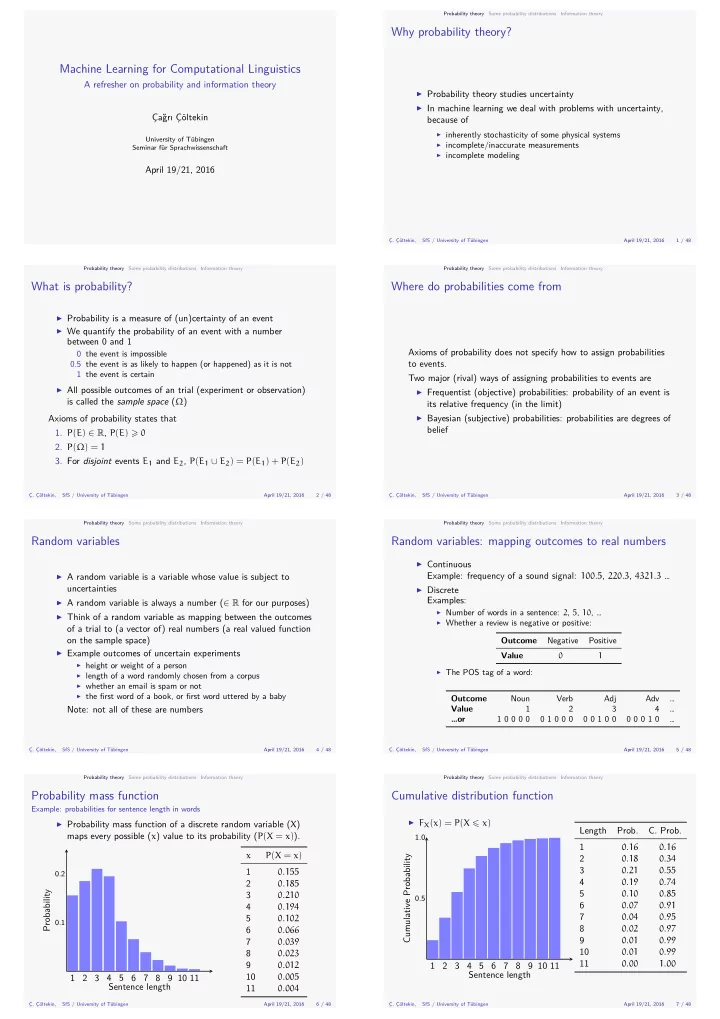
Probability mass function

Example: probabilities for sentence length in words

▶ Probability mass function of a discrete random variable (X)

maps every possible (x) value to its probability (P(X = x)). Probability Sentence length

0.1 0.2

1 2 3 4 5 6 7 8 9 10 11 x P(X = x) 1 0.155 2 0.185 3 0.210 4 0.194 5 0.102 6 0.066 7 0.039 8 0.023 9 0.012 10 0.005 11 0.004

Ç. Çöltekin, SfS / University of Tübingen April 19/21, 2016 6 / 48 Probability theory Some probability distributions Information theory

Cumulative distribution function

▶ FX(x) = P(X ⩽ x)

Cumulative Probability Sentence length

0.5 1.0

1 2 3 4 5 6 7 8 9 10 11 Length Prob.

• C. Prob.

1 0.16 0.16 2 0.18 0.34 3 0.21 0.55 4 0.19 0.74 5 0.10 0.85 6 0.07 0.91 7 0.04 0.95 8 0.02 0.97 9 0.01 0.99 10 0.01 0.99 11 0.00 1.00

Ç. Çöltekin, SfS / University of Tübingen April 19/21, 2016 7 / 48

SLIDE 2

Probability theory Some probability distributions Information theory

Expected value

▶ Expected value (mean) of a random variable X is,

E[X] = µ =

n

∑

i=1

P(xi)xi = P(x1)x1 +P(x2)x2 +. . .+P(xn)xn

▶ More generally, expected value of a function of X is

E[f(X)] =

n

∑

i=1

P(xi)f(xi)

▶ Expected value is an important measure of central tendency ▶ Note: it is not the ‘most likely’ value ▶ Expected value is linear

E[aX + bY] = aE[X] + bE[Y]

Ç. Çöltekin, SfS / University of Tübingen April 19/21, 2016 8 / 48 Probability theory Some probability distributions Information theory

Variance and standard deviation

▶ Variance of a random variable X is,

Var(X) = σ2 =

n

∑

i=1

P(xi)(xi − µ)2 = E[X2] − (E[X])2

▶ It is a measure of spread, divergence from the central tendency ▶ The square root of variance is called standard deviation

σ =

• n

∑

i=1

( P(xi)x2

i

) − µ2

▶ Standard deviation is in the same units as the values of the

random variable

▶ Variance is not linear: σ2 X+Y ̸= σ2 X + σ2 Y (neither the σ)

Ç. Çöltekin, SfS / University of Tübingen April 19/21, 2016 9 / 48 Probability theory Some probability distributions Information theory

Short divergence: Chebyshev’s inequality

For any probability distribution, and k > 1, P(|x − µ| > kσ) ⩽ 1 k2 Distance from µ 2σ 3σ 5σ 10σ 100σ Probability 0.25 0.11 0.04 0.01 0.0001 This also shows why standardizing values of random variables, z = x − µ σ makes sense (the normalized quantity is often called the z-score).

Ç. Çöltekin, SfS / University of Tübingen April 19/21, 2016 10 / 48 Probability theory Some probability distributions Information theory

Median and mode of a random variable

Median is the mid-point of a distribution. Median of a random variable is defjned as the number m that satisfjes P(X ⩽ m) ⩾ 1 2 and P(X ⩾ m) ⩾ 1 2

▶ Median of 1, 4, 5, 8, 10 is 5 ▶ Median of 1, 4, 5, 7, 8, 10 is 6

Mode is the value that occurs most often in the data.

▶ Modes appear as peaks in probability mass (or density)

functions

▶ Mode of 1, 4, 4, 8, 10 is 4 ▶ Modes of 1, 4, 4, 8, 9, 9 are 4 and 9

Ç. Çöltekin, SfS / University of Tübingen April 19/21, 2016 11 / 48 Probability theory Some probability distributions Information theory

Mode, median, mean, standard deviation

Visualization on sentence length example

Probability Sentence length

0.1 0.2

1 2 3 4 5 6 7 8 9 10 11 mode = median = 3.0 µ = 3.56 σ = 2 . 9

Ç. Çöltekin, SfS / University of Tübingen April 19/21, 2016 12 / 48 Probability theory Some probability distributions Information theory

Probability distribution of letters

▶ We have a hypothetical language with 8 letters with the

following probabilities

Lett. a b c d e f g h Prob. 0.23 0.04 0.05 0.08 0.29 0.02 0.07 0.22

Probability Letter

0.1 0.2

e a h d g c b f

Ç. Çöltekin, SfS / University of Tübingen April 19/21, 2016 13 / 48 Probability theory Some probability distributions Information theory

Joint and marginal probability

Two random variables form a joint probability distribution. An examaple: consider the bigrams of letters in our earlier

• example. The joint distribution can be defjned with a table like the
• ne below.

a b c d e f g h a 0.04 0.02 0.02 0.03 0.05 0.01 0.02 0.06 0.23 b 0.01 0.00 0.00 0.00 0.01 0.00 0.00 0.01 0.04 c 0.02 0.00 0.00 0.00 0.01 0.00 0.00 0.01 0.05 d 0.02 0.00 0.00 0.01 0.02 0.00 0.01 0.02 0.08 e 0.06 0.02 0.01 0.03 0.08 0.01 0.01 0.07 0.29 f 0.00 0.00 0.00 0.00 0.01 0.00 0.00 0.01 0.02 g 0.01 0.00 0.00 0.01 0.02 0.00 0.01 0.02 0.07 h 0.08 0.00 0.00 0.01 0.10 0.00 0.01 0.02 0.22 0.23 0.04 0.05 0.08 0.29 0.02 0.07 0.22

Ç. Çöltekin, SfS / University of Tübingen April 19/21, 2016 14 / 48 Probability theory Some probability distributions Information theory

Expected values of joint distributions

E[f(X, Y)] = ∑

x

∑

y

P(x, y)f(x, y) µX = E[X] = ∑

x

∑

y

P(x, y)x µY = E[Y] = ∑

x

∑

y

P(x, y)y We can simplify the notation by vector notation, for µ = (µx, µy), µ = ∑

x∈XY

xP(x) where vector x ranges over all possible combinations of the values

• f random variables X and Y.

Ç. Çöltekin, SfS / University of Tübingen April 19/21, 2016 15 / 48

SLIDE 3

Probability theory Some probability distributions Information theory

Variances of joint distributions

σ2

X =

∑

x

∑

y

P(x, y)(x − µX)2 σ2

Y =

∑

x

∑

y

P(x, y)(y − µY)2 σXY = ∑

x

∑

y

P(x, y)(x − µX)(y − µY)

▶ The last quantity is called covariance which indicates whether

the two variables vary together or not Again, using vector/matrix notation we can defjne the covariance matrix (Σ) as Σ = E[(x − µ)2]

Ç. Çöltekin, SfS / University of Tübingen April 19/21, 2016 16 / 48 Probability theory Some probability distributions Information theory

Covariance and the covariance matrix

Σ = [ σ2

X

σXY σYX σ2

Y

]

▶ The diagonal of the covariance matrix contains the variances

• f the individual variables

▶ Non-diagonal entries are the covariances of the corresponding

variables

▶ Covariance matrix is symmetric (σXY = σYX) ▶ For a joint distribution of k variables we have a covariance

matrix of size k × k

Ç. Çöltekin, SfS / University of Tübingen April 19/21, 2016 17 / 48 Probability theory Some probability distributions Information theory

Correlation

Correlation is a normalized version of covariance r = σXY σXσY Correlation coeffjcient (r) takes values between −1 and 1 1 Perfect positive correlation. (0, 1) positive correlation: x increases as y increases. 0 No correlation, variables are independent. (−1, 0) negative correlation: x decreases as y increases. −1 Perfect negative correlation. Note: like covariance, correlation is a symmetric measure.

Ç. Çöltekin, SfS / University of Tübingen April 19/21, 2016 18 / 48 Probability theory Some probability distributions Information theory

Correlation: visualization (1)

20 40 60 80 100 150 200 250

x y

r = 0.999

Ç. Çöltekin, SfS / University of Tübingen April 19/21, 2016 19 / 48 Probability theory Some probability distributions Information theory

Correlation: visualization (2)

20 40 60 80 50 100 150 200 250 300

x y

r = 0.809

Ç. Çöltekin, SfS / University of Tübingen April 19/21, 2016 20 / 48 Probability theory Some probability distributions Information theory

Correlation: visualization (3)

20 40 60 80

• 100
• 50

x y

r = -0.998

Ç. Çöltekin, SfS / University of Tübingen April 19/21, 2016 21 / 48 Probability theory Some probability distributions Information theory

Correlation: visualization (4)

20 40 60 80

• 200
• 150
• 100
• 50

50 100

x y

r = -0.688

Ç. Çöltekin, SfS / University of Tübingen April 19/21, 2016 22 / 48 Probability theory Some probability distributions Information theory

Correlation: visualization (5)

20 40 60 80 20 40 60 80 100

x y

r = 0.123

Ç. Çöltekin, SfS / University of Tübingen April 19/21, 2016 23 / 48

SLIDE 4

Probability theory Some probability distributions Information theory

Correlation and independence

▶ Statistical (in)dependence is an important concept (in ML) ▶ The covariance (or correlation) of independent random

variables are 0

▶ The reverse is not true: 0 correlation does not imply

independence

▶ Correlation measures a linear dependence (relationship)

between two variables, non-linear dependence may not be measured by covariance

Ç. Çöltekin, SfS / University of Tübingen April 19/21, 2016 24 / 48 Probability theory Some probability distributions Information theory

Conditional probability

In our letter bigram example, given that we know that the fjrst letter is e, what is the probability of second letter being d?

a b c d e f g h a 0.04 0.02 0.02 0.03 0.05 0.01 0.02 0.06 0.23 b 0.01 0.00 0.00 0.00 0.01 0.00 0.00 0.01 0.04 c 0.02 0.00 0.00 0.00 0.01 0.00 0.00 0.01 0.05 d 0.02 0.00 0.00 0.01 0.02 0.00 0.01 0.02 0.08 e 0.06 0.02 0.01 0.03 0.08 0.01 0.01 0.07 0.29 f 0.00 0.00 0.00 0.00 0.01 0.00 0.00 0.01 0.02 g 0.01 0.00 0.00 0.01 0.02 0.00 0.01 0.02 0.07 h 0.08 0.00 0.00 0.01 0.10 0.00 0.01 0.02 0.22 0.23 0.04 0.05 0.08 0.29 0.02 0.07 0.22

P(L1 = e, L2 = d) = 0.025940365 P(L1 = e) = 0.28605090 P(L2 = d|L1 = e) = P(L1 = e, L2 = d) P(L1 = e)

Ç. Çöltekin, SfS / University of Tübingen April 19/21, 2016 25 / 48 Probability theory Some probability distributions Information theory

Conditional probability (2)

In terms of probability mass (or density) functions, P(X|Y) = P(X, Y) P(Y) If two variables are independent, knowing the outcome of one does not afgect the probability of the other variable: P(X|Y) = P(X) P(X, Y) = P(X)P(Y) More notes on notation/interpretation: P(X = x, Y = y) Probability that X = x and Y = y at the same time (joint probability) P(Y = y) Probability of Y = y, for any value of X (∑

x∈X P(X = x, Y = y)) (marginal probability)

P(X = x|Y = y) Knowing that we Y = y, P(X = x) (conditional probability)

Ç. Çöltekin, SfS / University of Tübingen April 19/21, 2016 26 / 48 Probability theory Some probability distributions Information theory

Chain rule

We rewrite the relation between the joint and the conditional probability as P(X, Y) = P(X|Y)P(Y) We can also write the same quantity as, P(X, Y) = P(Y|X)P(X) For more than two variables, one can write P(X, Y, Z) = P(Z|X, Y)P(Y|X)P(X) = P(X|Y, Z)P(Y|Z)P(Z) = . . . In general, for any number of random variables, we can write P(X1, X2, . . . , Xn) = P(X1|X2, . . . , Xn)P(X2, . . . , Xn)

Ç. Çöltekin, SfS / University of Tübingen April 19/21, 2016 27 / 48 Probability theory Some probability distributions Information theory

Conditional independence

If two random variables are conditionally independent: P(X, Y|Z) = P(X|Z)P(Y|Z) This is often used for simplifying the ML systems. For example in spam fjltering with Naive Bayes classifjer, we are interested in P(w1, w2, w3|spam) = P(w1|w2, w3, spam)P(w2|w3, spam)P(w3|spam) with the assumption that occurence of words are independent of each other given we know the email is spam or not, P(w1, w2, w3|spam) = P(w1|spam)P(w2|spam)P(w3|spam)

Ç. Çöltekin, SfS / University of Tübingen April 19/21, 2016 28 / 48 Probability theory Some probability distributions Information theory

Bayes’ rule

P(X|Y) = P(Y|X)P(X) P(Y)

▶ This is a direct result of rules of probability ▶ It is often useful as it ‘inverts’ the conditional probabilities ▶ The term P(X), is called prior ▶ The term P(Y|X), is called likelihood ▶ The term P(X|Y), is called posterior

Ç. Çöltekin, SfS / University of Tübingen April 19/21, 2016 29 / 48 Probability theory Some probability distributions Information theory

Example application of Bayes’ rule

We use a test t to determine a patient has condition/illness c

▶ If a patient has c test is positive 99% of the time:

P(t|c) = 0.99

▶ What is the probability that a patient has c given t? ▶ …or more correctly, can you calculate this probability? ▶ We need to know two more quantities. Let’s assume

P(c) = 0.00001 and P(t|¬c)) = 0.02 P(c|t) = P(t|c)P(c) P(t) = P(t|c)P(c) P(t|c)P(c) + P(t|¬c)P(¬c) = 0.0005

Ç. Çöltekin, SfS / University of Tübingen April 19/21, 2016 30 / 48 Probability theory Some probability distributions Information theory

Continuous random variables

The rules and quantities we discussed above apply to continuous random variables with some difgerences

▶ For continuous variables, P(X = x) = 0 ▶ We cannot talk about probability of the variable being equal

to a single real number

▶ But we can defjne probabilities of ranges ▶ For all formulas we have seen so far, replace summation with

integrals

Ç. Çöltekin, SfS / University of Tübingen April 19/21, 2016 31 / 48

SLIDE 5

Probability theory Some probability distributions Information theory

Probability density function

• 2
• 1

1 2 0.0 0.5 1.0 1.5 x Density (p(x)) x ∼ N(0, 1

4)

Ç. Çöltekin, SfS / University of Tübingen April 19/21, 2016 32 / 48 Probability theory Some probability distributions Information theory

Continuous random variables: some defjnitions

▶ Probability of a range:

P(a < X < b) = ∫ b

a

p(x)dx

▶ Joint probability density

p(X, Y) = P(X|Y)P(Y) = P(Y|X)P(X)

▶ Marginal probability

P(X) = ∫ ∞

−∞

p(x, y)dy

Ç. Çöltekin, SfS / University of Tübingen April 19/21, 2016 33 / 48 Probability theory Some probability distributions Information theory

Uniform distribution (discrete)

▶ A uniform distribution

assigns equal probabilities to all values in range [a, b], where a and b are the parameters of the distribution

▶ Probabilities of the values

• utside range is 0

▶ µ = 1 a−b+1 ▶ σ2 = (b−a+1)2 12 ▶ There is also an analogous

continuous uniform distribution x ∼ Unif(a, b) n = a + b + 1

1 n

…

a b

Ç. Çöltekin, SfS / University of Tübingen April 19/21, 2016 34 / 48 Probability theory Some probability distributions Information theory

Bernoulli distribution

Bernoulli distribution characterizes simple random experiments with two outcomes

▶ Coin fmip: heads or tails ▶ Spam detection: spam or not ▶ Predicting gender: female or male

We denote (arbitrarily) one of the possible values with 1 (often called a success), the other with 0 (often called a failure) P(X = 1) = p P(X = 0) = 1 − p µX = p σ2

X = p(1 − p)

Ç. Çöltekin, SfS / University of Tübingen April 19/21, 2016 35 / 48 Probability theory Some probability distributions Information theory

Binomial distribution

Binomial distribution is a generalization of Bernoulli distribution to n trials, the value of the random variable is the number of ‘successes’ in the experiment P(X = k) = (n k ) pk(1 − p)k µX = np σ2

X = np(1 − p)

Ç. Çöltekin, SfS / University of Tübingen April 19/21, 2016 36 / 48 Probability theory Some probability distributions Information theory

Categorical distribution

▶ Extension of Bernoulli to k mutually exclusive outcomes ▶ For any k-way event, distribution is parametrized by k

parameters p1, . . . , pk (k − 1 independent parameters) where

k

∑

i=1

pi = 1 E[xi] = pi Var(xi) = pi(1 − pi)

▶ Similar to Bernoulli–binomial generalization, multinomial

distribution is the generalization of categorical distribution to n trials

Ç. Çöltekin, SfS / University of Tübingen April 19/21, 2016 37 / 48 Probability theory Some probability distributions Information theory

Gaussian (or normal) distribution

• 4
• 2

2 4 0.0 0.1 0.2 0.3 0.4 x Density p(x; µ, σ2) =

1 σ √ 2πe− (x−µ)2

2σ2

x ∼ N(µ, σ2)

Ç. Çöltekin, SfS / University of Tübingen April 19/21, 2016 38 / 48 Probability theory Some probability distributions Information theory

Short detour: central limit theorem

Central limit theorem (CLT) states that the sum of a large number

• f independent and identically distributed variables (i.i.d.)is

normally distributed.

▶ Expected value (average) of means of samples from any

distribution will be distributed normally

▶ Many (inference) methods in statistics and machine learning

works because of this fact

Ç. Çöltekin, SfS / University of Tübingen April 19/21, 2016 39 / 48

SLIDE 6

Probability theory Some probability distributions Information theory

Beta distribution

▶ Beta distribution is defjned

in range [0, 1]

▶ A common use is the

random variables whose values are probabilities

▶ It is characterized by two

parameters α and β

▶ Particularly important in

Bayesian methods as a conjugate prior of Bernoulli and Binomial distributions 0.0 0.2 0.4 0.6 0.8 1.0 1 2 3 4 x Density x ∼ Beta(0.5, 0.5) x ∼ Beta(1.0, 1.0) x ∼ Beta(2.0, 5.0) x ∼ Beta(5.0, 2.0)

▶ Dirichlet distribution generalizes Beta to k-dimensional vectors

whose components are in range (0, 1) and ∥x∥1 = 1.

Ç. Çöltekin, SfS / University of Tübingen April 19/21, 2016 40 / 48 Probability theory Some probability distributions Information theory

Information theory

▶ Information theory is concerned with measurement, storage

and transmission of information

▶ I has its roots in communication theory, but applied to many

difgerent fjelds including machine learning

▶ We will revisit some of the major measures here

Ç. Çöltekin, SfS / University of Tübingen April 19/21, 2016 41 / 48 Probability theory Some probability distributions Information theory

Entropy and Information

Entropy is a measure of uncertainty of a random variable: H(X) = − ∑

x

P(x) log2 P(x)

▶ Unit of information above is bit ▶ It generalizes to continuous distributions as well (replace sum

with integral)

▶ Note: H(x) = E[log2 1/p]

Ç. Çöltekin, SfS / University of Tübingen April 19/21, 2016 42 / 48 Probability theory Some probability distributions Information theory

Example: entropy letter distributions

Take our example letter distribution:

Lett. a b c d e f g h Prob. 0.23 0.04 0.05 0.08 0.29 0.02 0.07 0.22

H(X) = − (0.23 log2 0.23 + 0.04log20.04 + . . . + 0.22 log2 0.22) = 2.57

▶ If the letters were distributed uniformly (all having P(x) = 1 8),

H(X) = 3

▶ If only one of the letters were possible, H(X) = 0

Ç. Çöltekin, SfS / University of Tübingen April 19/21, 2016 43 / 48 Probability theory Some probability distributions Information theory

Example: entropy of a Bernoulli distribution

0.0 0.2 0.4 0.6 0.8 1.0 0.2 0.4 0.6 0.8 1.0 p H

Ç. Çöltekin, SfS / University of Tübingen April 19/21, 2016 44 / 48 Probability theory Some probability distributions Information theory

Relative entropy / KL divergence / information gain

For two distribution p and q defjned on the same variable, Kullback–Leibler divergence of q from p (or relative entropy of p given q) is defjned as DKL = (p(X)∥q(X)) = ∑

i

p(x) log2 p(x) q(x)

▶ DKL measures the amount of information lost when q is used

for approximating p

▶ Used for measuring difgerence between two distributions ▶ Note: it is not symmetric (not a distance measure)

Ç. Çöltekin, SfS / University of Tübingen April 19/21, 2016 45 / 48 Probability theory Some probability distributions Information theory

Mutual information

Mutual information measures mutual dependence between two random variables I(X, Y) = ∑

x

∑

y

P(x, y)log2 P(x, y) P(x)P(y)

▶ If variables are statistically independent I(X, Y) = 0 ▶ It is equivalent to DKL(P(X, Y)∥P(X)P(Y)) ▶ Mutual information is symmetric I(X, Y) = I(Y, X) ▶ Unlike correlation, mutual information is also defjned for

discrete variables

Ç. Çöltekin, SfS / University of Tübingen April 19/21, 2016 46 / 48 Probability theory Some probability distributions Information theory

Pointwise mutual information

Pointwise mutual information (PMI) between two events (outcomes) is defjned as PMI(x, y) = log2 P(x, y) P(x)P(y)

▶ PMI is often used as a measure of association (e.g., between

words) in (computational) linguistics

▶ Expected value of PMI is mutual information

Ç. Çöltekin, SfS / University of Tübingen April 19/21, 2016 47 / 48

SLIDE 7

Probability theory Some probability distributions Information theory

Summary

▶ We went through a large number of topics from probability

and information theory

▶ We will revisit some of them when needed

Next: Tuesday Short introduction + Regression Thursday Regression (practical bits)

Ç. Çöltekin, SfS / University of Tübingen April 19/21, 2016 48 / 48

Further reading

▶ MacKay (2003) covers most of the topics discussed, in a way

quite relevant to machine learning. The complete book is available freely online (see the link below)

▶ See Grinstead and Snell (2012) a more conventional

introduction to probability theory. This book is also freely available

▶ For an infmuential, but not quite conventional approach, see

Jaynes (2007)

Grinstead, Charles Miller and James Laurie Snell (2012). Introduction to probability. American Mathematical

• Society. isbn: 9780821894149. url:

http://www.dartmouth.edu/~chance/teaching_aids/books_articles/probability_book/book.html. Jaynes, Edwin T (2007). Probability Theory: The Logic of Science. Ed. by G. Larry Bretthorst. Cambridge University Press. isbn: 978-05-2159-271-0. MacKay, David J. C. (2003). Information Theory, Inference and Learning Algorithms. Cambridge University Press. isbn: 978-05-2164-298-9. url: http://www.inference.phy.cam.ac.uk/itprnn/book.html. Ç. Çöltekin, SfS / University of Tübingen April 19/21, 2016 A.1