m 2 s 2 2 ( ( x ) / 2 x / 2 ) ( ) - PDF document

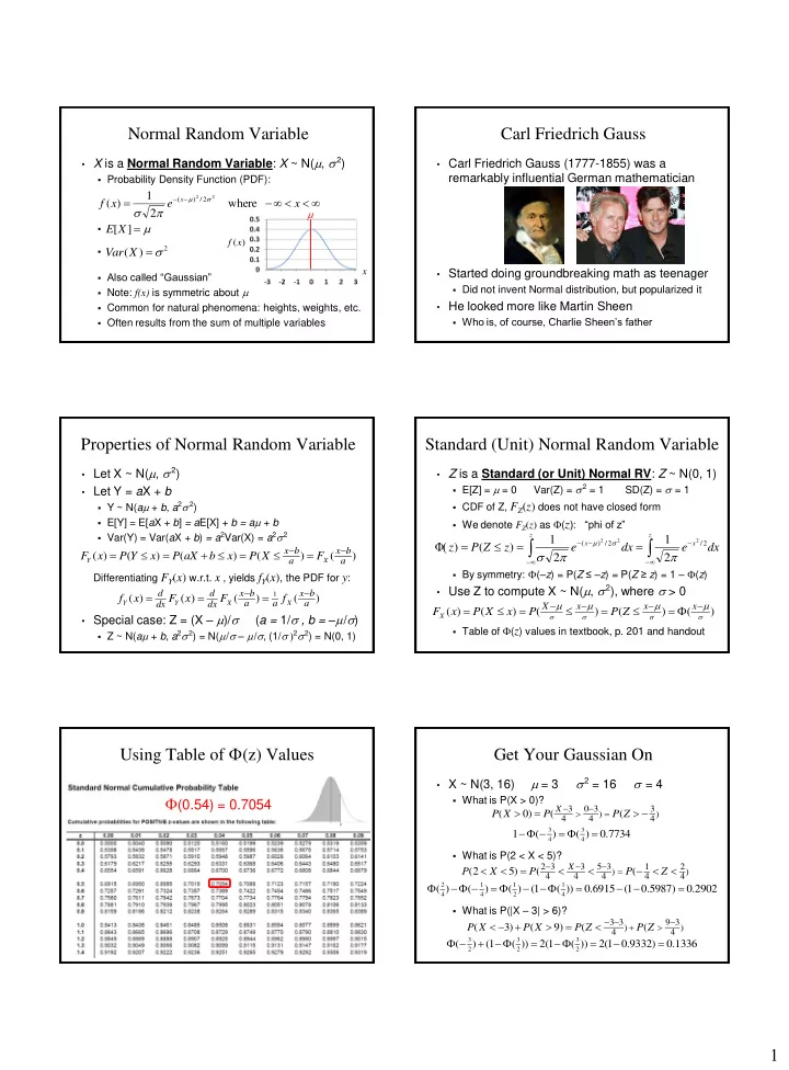
Normal Random Variable Carl Friedrich Gauss • X is a Normal Random Variable : X ~ N( m , s 2 ) • Carl Friedrich Gauss (1777-1855) was a remarkably influential German mathematician  Probability Density Function (PDF): 1 2 2    m s 2      ( x ) / f ( x ) e where x s  m 2  m  E [ X ] ( x ) f  s 2 ( )  Var X x • Started doing groundbreaking math as teenager  Also called “Gaussian”  Note: f(x) is symmetric about m  Did not invent Normal distribution, but popularized it • He looked more like Martin Sheen  Common for natural phenomena: heights, weights, etc.  Who is, of course, Charlie Sheen’s father  Often results from the sum of multiple variables Properties of Normal Random Variable Standard (Unit) Normal Random Variable • Let X ~ N( m , s 2 ) • Z is a Standard (or Unit) Normal RV : Z ~ N(0, 1) Var(Z) = s 2 = 1  E[Z] = m = 0 SD(Z) = s = 1 • Let Y = a X + b  Y ~ N( a m + b , a 2 s 2 )  CDF of Z, F Z ( z ) does not have closed form  E[Y] = E[ a X + b ] = a E[X] + b = a m + b  We denote F Z ( z ) as  ( z ): “phi of z”  Var(Y) = Var( a X + b ) = a 2 Var(X) = a 2 s 2 z z 1 1        m 2 s 2   2 Φ( ( x ) / 2 x / 2 ) ( ) z P Z z e dx e dx          x b  x b s   ( ) ( ) ( ) ( ) ( ) F x P Y x P aX b x P X F 2 2 Y a X a      By symmetry:  ( – z ) = P( Z ≤ – z ) = P( Z ≥ z ) = 1 –  ( z ) Differentiating F Y ( x ) w.r.t. x , yields f Y ( x ) , the PDF for y : • Use Z to compute X ~ N( m , s 2 ), where s > 0    d  d x b  x b 1 ( ) ( ) ( ) ( ) f x F x F f  m  m  m  m Y dx Y dx X a a X a    X  x   x   x ( ) ( ) ( ) ( ) ( ) F X x P X x P P Z • Special case: Z = (X – m )/ s ( a = 1/ s , b = – m / s ) s s s s  Table of  ( z ) values in textbook, p. 201 and handout  Z ~ N( a m + b , a 2 s 2 ) = N( m / s – m / s , (1/ s ) 2 s 2 ) = N(0, 1) Using Table of  (z) Values Get Your Gaussian On m = 3 s 2 = 16 s = 4 • X ~ N(3, 16)  (0.54) = 0.7054  What is P(X > 0)?   3 0 3 3   X     P ( X 0 ) P ( P ( Z ) ) 4 4 4    3   3  1 ( ) ( ) 0 . 7734 4 4  What is P(2 < X < 5)?    2 3 3 5 3 1 2     X     ( 2 5 ) (  ( P X P ) P Z ) 4 4 4 4 4              2 1 1 1 ( ) ( ) ( ) ( 1 ( )) 0 . 6915 ( 1 0 . 5987 ) 0 . 2902 4 4 2 4  What is P(|X – 3| > 6)?          3 3 9 3 ( 3 ) ( 9 ) (  (  P X P X P Z ) P Z ) 4 4   3    3    3    ( ) ( 1 ( )) 2 ( 1 ( )) 2 ( 1 0 . 9332 ) 0 . 1336 2 2 2 1

Noisy Wires Normal Approximation to Binomial • Send voltage of 2 or -2 on wire (to denote 1 or 0) • X ~ Bin( n , p ) Var(X) = np (1 – p )  X = voltage sent  E[X] = np  R = voltage received = X + Y, where noise Y ~ N(0, 1)  Poisson approx. good: n large (> 20), p small (< 0.05)  For large n: X  Y ~ N(E[X], Var(X)) = N( np , np (1 – p ))  Decode R: if (R ≥ 0.5) then 1, else 0  Normal approx. good : Var(X) = np (1 – p ) ≥ 10  What is P(error after decoding | original bit = 1)?              ) P ( 2 Y 0 . 5 ) P ( Y 1 . 5 ) ( 1 . 5 ) 1 ( 1 . 5 ) 0 . 0668         0 . 5 0 . 5 k np k np 1 1               ( ) P X k P k Y k     2 2   ( 1 ) ( 1 )  np p   np p   What is P(error after decoding | original bit = 0)?           DeMoivre-Laplace Limit Theorem: ( 2 0 . 5 ) ( 2 . 5 ) 1 ( 2 . 5 ) 0 . 0062 P Y P Y o S n : number of successes (with prob. p ) in n independent trials    S np              n P a n b ( b ) ( a )    ( 1 )  np p  Comparison when n = 100, p = 0.5 Faulty Endorsements • 100 people placed on special diet  X = # people on diet whose cholesterol decreases  Doctor will endorse diet if X ≥ 65  What is P(doctor endorses diet | diet has no effect)?  X ~ Bin(100, 0.5) P(X = k )    – p) – p) 50 1 25 1 5 np np( np(  Use Normal approximation: Y ~ N(50, 25)    P ( X 65 ) P ( Y 64 . 5 )  )     Y 50  64 . 5 50     ( 64 . 5 ) 1 ( 2 . 9 ) 0 . 0019 P Y P 5 5  Using Binomial:   ( 65 ) 0 . 0018 P X k Stanford Admissions Exponential Random Variable • X is an Exponential RV : X ~ Exp( l ) Rate: l > 0 • Stanford accepts 2480 students  Each accepted student has 68% chance of attending  Probability Density Function (PDF):   X = # students who will attend. X ~ Bin(2480, 0.68) l  l  x e if x 0        ( ) where x f x  What is P(X > 1745)?   0 if x 0    – p) – p) np 1686 . 4 np( 1 539 . 65 np( 1 23 . 23 1  [ ]  E X  Use Normal approximation: Y ~ N(1686.4, 539.65) l f ( x )    P ( X 1745 ) P ( Y 1745 . 5 ) 1  ( ) Var X  )  l x 2   1686 . 4 1745 . 5 1686 . 4   Y      P ( Y 1745 . 5 ) P 1 ( 2 . 54 ) 0 . 0055 23 . 23 23 . 23  Cumulative distribution function (CDF), F (X) = P( X  x ):    l  x ( ) 1 where 0 F x e x  Using Binomial:    Represents time until some event P ( X 1745 ) 0 . 0053 o Earthquake, request to web server, end cell phone contract, etc. 2

Exponential is “Memoryless” Visits to Web Site • X = time until some event occurs • Say a visitor to your web leaves after X minutes  X ~ Exp( l )  On average, visitors leave site after 5 minutes  What is P(X > s + t | X > s)?  Assume length of stay is Exponentially distributed  X ~ Exp( l = 1/5), since E[X] = 1/ l = 5      ( and ) ( ) P X s t X s P X s t      P ( X s t | X s )    What is P(X > 10)? P ( X s ) P ( X s )        l         l  10 2 ( s t ) ( 10 ) 1 ( 10 ) 1 ( 1 ) 0 . 1353 ( ) 1 ( ) P X F e e P X s t F s t e     l     t e 1 F ( t ) P ( X t )    l s P ( X s ) 1 F ( s ) e  What is P(10 < X < 20)?      So, ( | ) ( ) P X s t X s P X t         4   2  P ( 10 X 20 ) F ( 20 ) F ( 10 ) ( 1 e ) ( 1 e ) 0 . 1170  After initial period of time s , P(X > t |  ) for waiting another t units of time until event is same as at start  “Memoryless” = no impact from preceding period s Replacing Your Laptop A Little Calculus Review • X = # hours of use until your laptop dies • Product rule for derivatives:  )      On average, laptops die after 5000 hours of use d ( u v du v u dv  X ~ Exp( l = 1/5000), since E[X] = 1/ l = 5000 • Derivative and integral of exponential:  You use your laptop 5 hours/day.  ( u )  d e du u u  e du e u  What is P(your laptop lasts 4 years)? e dx dx  That is: P(X > (5)(365)(4) = 7300)           • Integration by parts: 7300 / 5000 1 . 46 P ( X 7300 ) 1 F ( 7300 ) 1 ( 1 e ) e 0 . 2322           ( ) d u v u v v du u dv  Better plan ahead... especially if you are coterming:              1 . 825 u dv u v v du P ( X 9125 ) 1 F ( 9125 ) e 0 . 1612 (5 year plan)       2 . 19 ( 10950 ) 1 ( 10950 ) 0 . 1119 (6 year plan) P X F e And Now, Some Calculus Practice • Compute n -th moment of Exponential distribution    l  l n n x E [ X ] x e dx 0  Step 1: don’t panic, think happy thoughts, recall...  Step 2: find u and v (and du and dv ):     l n x u x v e    l  l n 1 x du nx dx dv e dx  Step 3: substitute (a.k.a. “plug and chug”)        l  l        l    l 1 n x n x n x u dv x e dx u v v du x e nx e dx       l    l   n  l  l  n  n n x n 1 x n 1 x n 1 E [ X ] x e nx e dx 0 x e dx E [ X ] l l 0 1 2 1 2      0 2 Base case : E [ X ] E [ 1 ] 1 , so E [ X ] E [ X ] ,... , l l l l 2 3