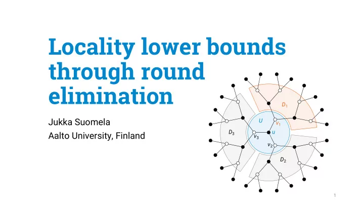
[PPT] - Locality lower bounds through round elimination D 1 Jukka Suomela PowerPoint Presentation

SLIDE 1

Locality lower bounds through round elimination

Jukka Suomela Aalto University, Finland

1

u v1 U v2 v3 D3 D2 D1

SLIDE 2

Joint work with

Alkida Balliu
Sebastian Brandt
Orr Fischer
Juho Hirvonen
Barbara Keller
Tuomo Lempiäinen
Dennis Olivetti
Mikaël Rabie
Joel Rybicki
Jara Uitto

2

SLIDE 3

Joint work with

Alkida Balliu
Sebastian Brandt
Orr Fischer
Juho Hirvonen
Barbara Keller
Tuomo Lempiäinen
Dennis Olivetti
Mikaël Rabie
Joel Rybicki
Jara Uitto

3

SLIDE 4

4

Locality = how far do I need to see to produce my own part of the solution?

SLIDE 5

5

I will output black

Locality = how far do I need to see to produce my own part of the solution?

SLIDE 6

6

I will output

range

I will output blue I will output black

Locality = how far do I need to see to produce my own part of the solution?

SLIDE 7

7

Locality = how far do I need to see to produce my own part of the solution?

Local outputs form a globally consistent solution

SLIDE 8

Locality: formalization

“LOCAL” model of distributed computing:
graph = communication network
node = processor
edge = communication link
all nodes have unique identifiers
time = number of communication rounds
round = nodes exchange messages with all neighbors
1 communication round: all nodes can learn everything within distance 1
T communication rounds: all nodes can learn everything within distance T
Time = distance

8

SLIDE 9

Locality: examples

Setting: graph with n nodes, maximum degree Δ = O(1)
Maximal independent set:

Θ(log* n) randomized, Θ(log* n) deterministic

Sinkless orientation:

Θ(log log n) randomized, Θ(log n) deterministic

orient edges such that all nodes of degree ≥ 3 have outdegree ≥ 1

9

SLIDE 10

How to study locality?

Proving locality upper & lower bounds

10

SLIDE 11

Locality: proving upper bounds

Find a function that maps local neighborhoods to local outputs
Design a fast distributed message-passing algorithm
Design a slow distributed algorithm and apply “speedup”

arguments to turn it into a fast distributed algorithm

e.g. o(n) → O(log* n) for “LCL problems” in cycles
Design a fast centralized sequential algorithm model and turn it

into a fast distributed algorithm

e.g. greedy strategy → SLOCAL algorithm → LOCAL algorithm

11

SLIDE 12

Locality: proving lower bounds

Indistinguishability
same local view → same output
Adaptive constructions
inductively construct a bad input

for this specific algorithm

Ramsey-type arguments
“monochromatic set” ≈ bad choice of identifiers
Speedup & derandomization arguments and reductions
locality R → locality R’ → not possible

12

SLIDE 13

Locality: proving lower bounds

Indistinguishability
same local view → same output
Adaptive constructions
inductively construct a bad input

for this specific algorithm

Ramsey-type arguments
“monochromatic set” ≈ bad choice of identifiers
Speedup & derandomization arguments and reductions
locality R → locality R’ → not possible

13

Today’s focus: “round elimination” technique for proving locality lower bounds

SLIDE 14

Round elimination

14

SLIDE 15

Round elimination technique

Given:
algorithm A0 solves problem P0 in T rounds
We construct:
algorithm A1 solves problem P1 in T − 1 rounds
algorithm A2 solves problem P2 in T − 2 rounds
algorithm A3 solves problem P3 in T − 3 rounds

…

algorithm AT solves problem PT in 0 rounds
But PT is nontrivial, so A0 cannot exist

15

SLIDE 16

Linial (1987, 1992): coloring cycles

Given:
algorithm A0 solves 3-coloring in T = o(log* n) rounds
We construct:
algorithm A1 solves 23-coloring in T − 1 rounds
algorithm A2 solves 223-coloring in T − 2 rounds
algorithm A3 solves 2223-coloring in T − 3 rounds

…

algorithm AT solves o(n)-coloring in 0 rounds
But o(n)-coloring is nontrivial, so A0 cannot exist

16

SLIDE 17

Brandt et al. (2016): sinkless orientation

Given:
algorithm A0 solves sinkless orientation in T = o(log n) rounds
We construct:
algorithm A1 solves sinkless coloring in T − 1 rounds
algorithm A2 solves sinkless orientation in T − 2 rounds
algorithm A3 solves sinkless coloring in T − 3 rounds

…

algorithm AT solves sinkless orientation in 0 rounds
But sinkless orientation is nontrivial, so A0 cannot exist

17

SLIDE 18

Round elimination can be automated

Good news: always possible for any graph problem P0

that is “locally checkable”

if problem P0 has complexity T, we can always find in a mechanical

manner problem P1 that has complexity T − 1

holds for tree-like neighborhoods (e.g. high-girth graphs)
Bad news: this does not directly give a lower bound
P1 is not necessarily any natural graph problem
P1 does not necessarily have a small description
how do we prove that P1, P2, P3, etc. are nontrivial problems?

18

Brandt 2019

SLIDE 19

Round elimination and fixed points

Sometimes we are very lucky:
P0 = sinkless orientation
P1 = something (no need to understand it)
P2 = sinkless orientation
If you are feeling optimistic: just apply round elimination

in a mechanical manner for a small number of steps and see if your reach a fixed point or cycle

or you reach a well-known hard problem
Open question: exactly when does this happen?

19

SLIDE 20

Round elimination and “rounding down”

Sometimes some amount of creativity is needed:
P0 = k-coloring cycles
P1 = something complicated with 2k possible output labels
define: Q1 = 2k-coloring cycles
observation: solution to P1

implies a solution to Q1

20

P0 takes exactly T rounds → P1 takes exactly T − 1 rounds → Q1 takes at most T − 1 rounds → … → QT takes at most 0 rounds

SLIDE 21

How does it work?

21

SLIDE 22

Correct formalism

We will need the right formalism for the graph problems

that we study

It will look seemingly arbitrary and very restrictive at first
No worries, you can encode a broad range of locally

checkable problems in this formalism with some effort

maximal matching, maximal independent set,

vertex coloring, edge coloring, sinkless orientation …

22

SLIDE 23

Correct formalism: edge labeling in bipartite graphs

Assumption: input graph properly 2-colored (“white” / “black”)
Finite set of possible edge labels
White constraint:
feasible multiset of labels on

edges adjacent to a white node

Black constraint:
feasible multiset of labels on

edges adjacent to a black node

23

SLIDE 24

1 1 1 1 1 1 1 1 1 1 1 1 1 1 1 1

Example 1: sinkless orientation

Setting: bipartite 3-regular graphs
Encoding: use original graph
“0” = orient from white to black
“1” = orient from black to white
White constraint:
{0, 0, 0}, {0, 0, 1} or {0, 1, 1}
Black constraint:
{0, 0, 1}, {0, 1, 1} or {1, 1, 1}

24

SLIDE 25

H H H H H H H H H T T T T T T T T T

Example 2: sinkless orientation

Setting: 3-regular graphs
Encoding: subdivide edges
white = edge, black = node
“H” = head, “T” = tail
White constraint:
{H, T}
Black constraint:
{H, H, T}, {H, T, T} or {T, T, T}

25

SLIDE 26

2 1 1 1 1 3 3 3 2 1 1 2

1 2 3 1

Example 3: vertex coloring

Setting: 3-regular graphs
Encoding: subdivide edges
white = edge, black = node
“1”, “2”, “3” = color of incident black node
White constraint:
{1, 2} or {1, 3} or {2, 3}
Black constraint:
{1, 1, 1}, {2, 2, 2} or {3, 3, 3}

26

SLIDE 27

Correct formalism: white and black algorithms

White algorithm:
each white node produces labels on its incident edges
black nodes do nothing
satisfies white and black constraints
Black algorithm:
each black node produces labels on its incident edges
white nodes do nothing
satisfies white and black constraints
White and black complexity within ±1 round of each other

27

SLIDE 28

u v1 U v2 v3 D3 D2 D1

28

Round elimination

Given: white algorithm A that runs in T = 2 rounds

v1 in A sees U and D1

Construct: black algorithm A’ that runs in T − 1 = 1 rounds

u in A’ only sees U

A’: what is the set of possible

utputs of A for edge {u, v1}
ver all possible inputs in D1?

SLIDE 29

u v1 U v2 v3 D3 D2 D1

29

Round elimination

Given: white algorithm A that runs in T = 2 rounds

v1 in A sees U and D1

Construct: black algorithm A’ that runs in T − 1 = 1 rounds

u in A’ only sees U

A’: what is the set of possible

utputs of A for edge {u, v1}
ver all possible inputs in D1?

Why is this useful and nontrival? Can’t we get here the set of all possible outputs?

SLIDE 30

u v1 U v2 v3 D3 D2 D1

30

Example: edge coloring

Independence!

Assume there is some

extension D1 such that v1 labels {u, v1} green

Assume there is some

extension D2 such that v2 labels {u, v2} green

Then we can construct an

input in which both {u, v1} and {u, v2} are green

SLIDE 31

31

Example: edge coloring

Independence!

Assume there is some

extension D1 such that v1 labels {u, v1} green

Assume there is some

extension D2 such that v2 labels {u, v2} green

Then we can construct an

input in which both {u, v1} and {u, v2} are green

Algorithm A’ has to do something nontrivial Here: sets incident to black nodes have to be non-empty and disjoint They contain enough information so that we could recover a proper edge coloring in 1 extra round

SLIDE 32

Example: bipartite maximal matching

32

SLIDE 33

33

1 1 1 1 1 2 3 2 1 2 3 23 2 3 3 1 1 3 2 2 3 2 3 1 1 1 1 1 2 3 2 1 2 3 2 3 2 3 3 1 1 3 2 2 3 2 3 computer network with port numbering bipartite, 2-colored graph Δ-regular (here Δ = 3)

utput:

maximal matching

SLIDE 34

34

1 1 1 1 1 2 3 2 1 2 3 23 2 3 3 1 1 3 2 2 3 2 3

Very simple algorithm

unmatched white nodes: send proposal to port 1

SLIDE 35

35

1 1 1 1 1 2 3 2 1 2 3 23 2 3 3 1 1 3 2 2 3 2 3

Very simple algorithm

unmatched white nodes: send proposal to port 1 black nodes: accept the first proposal you get, reject everything else (break ties with port numbers)

SLIDE 36

36

1 1 1 1 1 2 3 2 1 2 3 23 2 3 3 1 1 3 2 2 3 2 3

Very simple algorithm

unmatched white nodes: send proposal to port 1 black nodes: accept the first proposal you get, reject everything else (break ties with port numbers)

SLIDE 37

37

1 1 1 1 1 2 3 2 1 2 3 23 2 3 3 1 1 3 2 2 3 2 3

Very simple algorithm

unmatched white nodes: send proposal to port 2

SLIDE 38

38

1 1 1 1 1 2 3 2 1 2 3 23 2 3 3 1 1 3 2 2 3 2 3

Very simple algorithm

unmatched white nodes: send proposal to port 2 black nodes: accept the first proposal you get, reject everything else (break ties with port numbers)

SLIDE 39

39

1 1 1 1 1 2 3 2 1 2 3 23 2 3 3 1 1 3 2 2 3 2 3

Very simple algorithm

unmatched white nodes: send proposal to port 2 black nodes: accept the first proposal you get, reject everything else (break ties with port numbers)

SLIDE 40

40

1 1 1 1 1 2 3 2 1 2 3 23 2 3 3 1 1 3 2 2 3 2 3

Very simple algorithm

unmatched white nodes: send proposal to port 3

SLIDE 41

41

1 1 1 1 1 2 3 2 1 2 3 23 2 3 3 1 1 3 2 2 3 2 3

Very simple algorithm

unmatched white nodes: send proposal to port 3 black nodes: accept the first proposal you get, reject everything else (break ties with port numbers)

SLIDE 42

42

1 1 1 1 1 2 3 2 1 2 3 23 2 3 3 1 1 3 2 2 3 2 3

Very simple algorithm

unmatched white nodes: send proposal to port 3 black nodes: accept the first proposal you get, reject everything else (break ties with port numbers)

SLIDE 43

43

1 1 1 1 1 2 3 2 1 2 3 23 2 3 3 1 1 3 2 2 3 2 3

Very simple algorithm

Finds a maximal matching in O(Δ) communication rounds Note: running time does not depend on n

SLIDE 44

Bipartite maximal matching

Maximal matching in very large 2-colored Δ-regular graphs
Simple algorithm: O(Δ) rounds, independently of n
Is this optimal?
o(Δ) rounds?
O(log Δ) rounds?
4 rounds??

44

SLIDE 45

Lower-bound proof

45

SLIDE 46

Round elimination technique for maximal matching

Given:
algorithm A0 solves problem P0 = maximal matching in T rounds
We construct:
algorithm A1 solves problem P1 in T − 1 rounds
algorithm A2 solves problem P2 in T − 2 rounds
algorithm A3 solves problem P3 in T − 3 rounds

…

algorithm AT solves problem PT in 0 rounds
But PT is nontrivial, so A0 cannot exist

46

What are the right problems Pi here?

SLIDE 47

Round elimination technique for maximal matching

Given:
algorithm A0 solves problem P0 = maximal matching in T rounds
We construct:
algorithm A1 solves problem P1 in T − 1 rounds
algorithm A2 solves problem P2 in T − 2 rounds
algorithm A3 solves problem P3 in T − 3 rounds

…

algorithm AT solves problem PT in 0 rounds
But PT is nontrivial, so A0 cannot exist

47

Let’s start with P0 …

SLIDE 48

48

O M M · · · · · M O O O P P · · · · · · · O O P

Representation for maximal matchings

white nodes “active”

utput one of these:

· 1 × M and (Δ−1) × O · Δ × P black nodes “passive” accept one of these: · 1 × M and (Δ−1) × {P , O} · Δ × O M = “matched” P = “pointer to matched” O = “other”

SLIDE 49

49

O M M · · · · · M O O O P P · · · · · · · O O P

Representation for maximal matchings

white nodes “active”

utput one of these:

· 1 × M and (Δ−1) × O · Δ × P black nodes “passive” accept one of these: · 1 × M and (Δ−1) × {P , O} · Δ × O M = “matched” P = “pointer to matched” O = “other”

W = MO∆−1 P∆,

B = M[PO]∆−1

O∆.

SLIDE 50

Parameterized problem family

50

W∆(x, y) = ⇣ MOd1

Pd⌘

OyXx, B∆(x, y) = ⇣ [MX][POX]d1

[OX]d⌘

[POX]y[MPOX]x,

where d = ∆ − x − y.

W = MO∆−1 P∆, B = M[PO]∆−1 O∆.

maximal matching “weak” matching

SLIDE 51

Main lemma

Given: A solves P(x, y) in T rounds
We can construct: A’ solves P(x + 1, y + x) in T − 1 rounds

51

W∆(x, y) = ⇣ MOd1

Pd⌘

OyXx, B∆(x, y) = ⇣ [MX][POX]d1

[OX]d⌘

[POX]y[MPOX]x,

where d = ∆ − x − y.

SLIDE 52

Putting things together

Maximal matching in o(Δ) rounds → “Δ1/2 matching” in o(Δ1/2) rounds → P(Δ1/2, 0) in o(Δ1/2) rounds → P(O(Δ1/2), o(Δ)) in 0 rounds → contradiction

52

What we really care about k-matching: select at most k edges per node Apply round elimination

(Δ1/2) times

SLIDE 53

Putting things together

Basic version:
deterministic lower bound, port-numbering model
Analyze what happens to local failure probability:
randomized lower bound, port-numbering model
With randomness you can construct unique identifiers w.h.p.:
randomized lower bound, LOCAL model
Fast deterministic → very fast randomized
stronger deterministic lower bound, LOCAL model

53

Proof technique does not work directly with unique IDs

SLIDE 54

Main results

Maximal matching and maximal independent set cannot be solved in

o(Δ + log log n / log log log n) rounds

with randomized algorithms

o(Δ + log n / log log n) rounds

with deterministic algorithms

54

Lower bound for MM implies a lower bound for MIS

SLIDE 55

55

log4 log n log n log n log log n log3 n log4 n log7 n log ∆ log ∆ log log ∆ ∆ log∗ n log3 log n s log n log log n log log n log log log n

Linial (1987, 1992), Naor (1991) Kuhn et al. (2004, 2016)

New New

Fischer (2017) Panconesi & Rizzi (2001) Barenboim et al. (2012, 2016) Israeli & Itai (1986) Fischer (2017) Hanckowiak et al. (2001) Hanckowiak et al. (1998)

deterministic randomized

Algorithms:

deterministic randomized

Lower bounds: Maximal matching, LOCAL model, O(f(Δ) + g(n))

FOCS 2019

SLIDE 56

Summary

Round elimination technique
Locality lower bounds for

a wide range of problems:

symmetry breaking in cycles
symmetry breaking in regular trees
algorithmic Lovász local lemma
maximal matching, maximal independent set …
And for a wide range of localities:
Ω(log* n), Ω(log log n), Ω(log n), Ω(log* Δ), Ω(Δ) …

56

u v1 U v2 v3 D3 D2 D1

SLIDE 57

Open questions

Lower bounds for volume complexity?
volume lower bounds for

sinkless orientation?

Lower bounds for problems related

to graph coloring?

when is partial/defective coloring “easy”

and when is it “hard”?

nontrivial lower bounds for (Δ+1)-coloring?
Exactly when do we get fixed points and why?

57

u v1 U v2 v3 D3 D2 D1