[PDF] - Local invariant feature Would like discussion section, more review PDF Document

SLIDE 1

CS 376: Computer Vision - lecture 12 2/27/2018 1

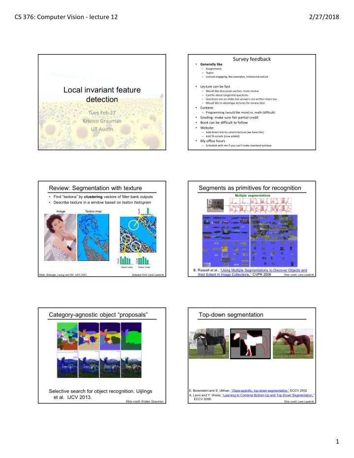
Local invariant feature detection

Tues Feb 27 Kristen Grauman UT Austin Survey feedback

Generally like

– Assignments – Topics – Lecture engaging, like examples, interactive nature

Lecture can be fast

– Would like discussion section, more review – Careful about tangential questions – Questions are on slides but answers not written there too – Would like to videotape lectures for review later

Content:

– Programming (would like more) vs. math (difficult)

Grading: make sure fair partial credit
Book can be difficult to follow
Website:

– Add direct link to current lecture (we have this) – Add TA emails (now added)

My office hours

– Schedule with me if you can’t make standard window

Review: Segmentation with texture

Find “textons” by clustering vectors of filter bank outputs
Describe texture in a window based on texton histogram

Malik, Belongie, Leung and Shi. IJCV 2001.

Texton map Image

Adapted from Lana Lazebnik

Texton index Texton index Count Count Count Texton index

Segments as primitives for recognition

B. Russell et al., “Using Multiple Segmentations to Discover Objects and

their Extent in Image Collections,” CVPR 2006

Multiple segmentations

Slide credit: Lana Lazebnik

Category-agnostic object “proposals”

Selective search for object recognition. Uijlings et al. IJCV 2013.

Slide credit: Kristen Grauman

Top-down segmentation

Slide credit: Lana Lazebnik

E. Borenstein and S. Ullman, “Class-specific, top-down segmentation,” ECCV 2002
A. Levin and Y. Weiss, “Learning to Combine Bottom-Up and Top-Down Segmentation,”

ECCV 2006.

SLIDE 2

CS 376: Computer Vision - lecture 12 2/27/2018 2

Top-down segmentation

E. Borenstein and S. Ullman, “Class-specific, top-down segmentation,” ECCV 2002
A. Levin and Y. Weiss, “Learning to Combine Bottom-Up and Top-Down Segmentation,”

ECCV 2006. Normalized cuts Top-down segmentation

Slide credit: Lana Lazebnik

Joint segmentation and recognition

Mask R-CNN, K. He et al., ICCV 2017

Video object segmentation

Goal: Extract all foreground objects  even those unseen during training  without manual intervention.

S. Jain et al., FusionSeg: Learning to combine motion and appearance for

fully automatic segmentation of generic objects in videos, CVPR 2017

http://vision.cs.utexas.edu/projects/fusionseg/

Slide credit: Kristen Grauman

Interactive image and video segmentation

[Jain & Grauman, HCOMP 2016] Click Carving https://github.com/suyogduttjain/click_carving

Results achieved with average of 2 user clicks

Slide credit: Kristen Grauman

Previously: Features and filters

Transforming and describing images; textures, colors, edges

Slide credit: Kristen Grauman

Previously: Grouping & fitting

[fig from Shi et al]

Clustering, segmentation, fitting; what parts belong together?

Slide credit: Kristen Grauman

SLIDE 3

CS 376: Computer Vision - lecture 12 2/27/2018 3

Now: Multiple views

Hartley and Zisserman Lowe

Matching, invariant features, stereo vision, instance recognition

Fei-Fei Li

Slide credit: Kristen Grauman

Important tool for multiple views: Local features

How to detect which local features to match? Multi-view matching relies on local feature correspondences.

Local features: main components

1) Detection: Identify the

interest points

2) Description:Extract vector

feature descriptor surrounding each interest point.

3) Matching: Determine

correspondence between descriptors in two views

] , , [

) 1 ( ) 1 ( 1 1 d

x x   x ] , , [

) 2 ( ) 2 ( 1 2 d

x x   x

Slide credit: Kristen Grauman

Local features: desired properties

Repeatability

– The same feature can be found in several images despite geometric and photometric transformations

Saliency

– Each feature has a distinctive description

Compactness and efficiency

– Many fewer features than image pixels

Locality

– A feature occupies a relatively small area of the image; robust to clutter and occlusion

Goal: interest operator repeatability

We want to detect (at least some of) the

same points in both images.

Yet we have to be able to run the detection

procedure independently per image.

No chance to find true matches!

Goal: descriptor distinctiveness

We want to be able to reliably determine

which point goes with which.

Must provide some invariance to geometric

and photometric differences between the two views.

?

SLIDE 4

CS 376: Computer Vision - lecture 12 2/27/2018 4

Local features: main components

1) Detection: Identify the

interest points

2) Description:Extract vector

feature descriptor surrounding each interest point.

3) Matching: Determine

correspondence between descriptors in two views

Slide credit: Kristen Grauman

What points would you choose?

Slide credit: Kristen Grauman

Detecting corners

Slide credit: Kristen Grauman

Compute “cornerness” response at every pixel.

Detecting corners

Slide credit: Kristen Grauman

Detecting corners

Slide credit: Kristen Grauman

Detecting local invariant features

Detection of interest points

– Harris corner detection – Scale invariant blob detection: LoG

(Next time: description of local patches)

SLIDE 5

CS 376: Computer Vision - lecture 12 2/27/2018 5

Corners as distinctive interest points

We should easily recognize the point by looking through a small window Shifting a window in any direction should give a large change in intensity

“edge”: no change along the edge direction “corner”: significant change in all directions “flat” region: no change in all directions

Slide credit: Alyosha Efros, Darya Frolova, Denis Simakov

       

y y y x y x x x

I I I I I I I I y x w M ) , (

x I I x    y I I y    y I x I I I

y x

     Corners as distinctive interest points

2 x 2 matrix of image derivatives (averaged in neighborhood of a point).

Notation:

First, consider an axis-aligned corner:

What does this matrix reveal?

                

2 1 2 2

 

y y x y x x

I I I I I I M

First, consider an axis-aligned corner: This means dominant gradient directions align with x or y axis Look for locations where both λ’s are large. If either λ is close to 0, then this is not corner-like.

What does this matrix reveal?

What if we have a corner that is not aligned with the image axes?

What does this matrix reveal?

Since M is symmetric, we have

T

X X M       

2 1

 

i i i

x Mx   The eigenvalues of M reveal the amount of intensity change in the two principal orthogonal gradient directions in the window.

Corner response function

“flat” region 1 and 2 are small; “edge”: 1 >> 2 2 >> 1 “corner”: 1 and 2 are large, 1 ~ 2;

Cornerness score (other variants possible)

SLIDE 6

CS 376: Computer Vision - lecture 12 2/27/2018 6

Harris corner detector

1) Compute M matrix for each image window to get their cornerness scores. 2) Find points whose surrounding window gave large corner response (f> threshold) 3) Take the points of local maxima, i.e., perform non-maximum suppression

Harris Detector: Steps Harris Detector: Steps

Compute corner response f

Harris Detector: Steps

Find points with large corner response: f > threshold

Harris Detector: Steps

Take only the points of local maxima of f

Harris Detector: Steps

SLIDE 7

CS 376: Computer Vision - lecture 12 2/27/2018 7

Properties of the Harris corner detector

Rotation invariant? Scale invariant?

T

X X M       

2 1

  Yes

Properties of the Harris corner detector

Rotation invariant? Scale invariant?

All points will be classified as edges

Corner !

Yes No

Scale invariant interest points

How can we independently select interest points in each image, such that the detections are repeatable across different scales?

Automatic Scale Selection

K. Grauman, B. Leibe

How to find corresponding patch sizes, with only one image in hand?

Automatic scale selection

Intuition:

Find scale that gives local maxima of some function

f in both position and scale. f

region size Image 1

f

region size Image 2

s1 s2

Automatic Scale Selection

Function responses for increasing scale (scale signature)
K. Grauman, B. Leibe

)) , ( (

1

 x I f

m

i i 

)) , ( (

1

 x I f

m

i i





SLIDE 8

CS 376: Computer Vision - lecture 12 2/27/2018 8 Automatic Scale Selection

Function responses for increasing scale (scale signature)
K. Grauman, B. Leibe

)) , ( (

1

 x I f

m

i i 

)) , ( (

1

 x I f

m

i i





Automatic Scale Selection

Function responses for increasing scale (scale signature)
K. Grauman, B. Leibe

)) , ( (

1

 x I f

m

i i 

)) , ( (

1

 x I f

m

i i





Automatic Scale Selection

Function responses for increasing scale (scale signature)
K. Grauman, B. Leibe

)) , ( (

1

 x I f

m

i i 

)) , ( (

1

 x I f

m

i i





Automatic Scale Selection

Function responses for increasing scale (scale signature)
K. Grauman, B. Leibe

)) , ( (

1

 x I f

m

i i 

)) , ( (

1

 x I f

m

i i





Automatic Scale Selection

Function responses for increasing scale (scale signature)
K. Grauman, B. Leibe

)) , ( (

1

 x I f

m

i i 

)) , ( (

1

  x I f

m

i i 

What can be the “signature” function?

SLIDE 9

CS 376: Computer Vision - lecture 12 2/27/2018 9

Blob detection in 2D

Laplacian of Gaussian: Circularly symmetric

perator for blob detection in 2D

2 2 2 2 2

y g x g g       

Blob detection in 2D: scale selection

Laplacian-of-Gaussian = “blob” detector

2 2 2 2 2

y g x g g       

filter scales

img1 img2 img3

Blob detection in 2D

We define the characteristic scale as the scale that produces peak of Laplacian response characteristic scale

Slide credit: Lana Lazebnik