
SLIDE 1
10/7/2015 1
Local features: detection and description
Kristen Grauman Thurs, Oct 8
Announcements
- Slides and pptfiles on course webpage
- A2 due this Friday
- A3 out next Tuesday, due Oct 30
- Midterm Oct 22
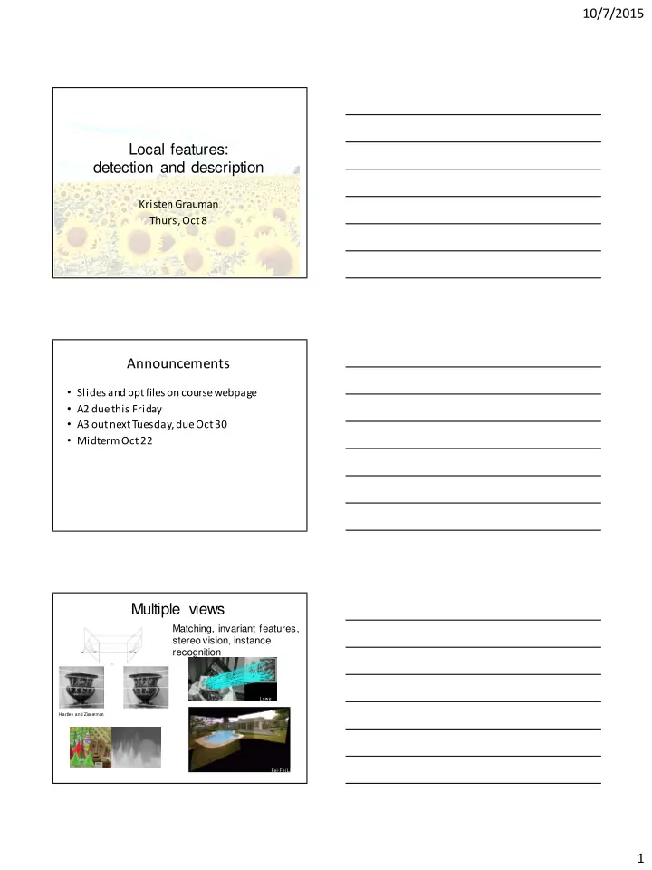
Multiple views
Hartley and Zisse rma n Lowe
Matching, invariant features, stereo vision, instance recognition
Fei-Fei Li