Loading Data Lecture 7 Running Assignment > F <- - - PowerPoint PPT Presentation

loading data
SMART_READER_LITE
LIVE PREVIEW

Loading Data Lecture 7 Running Assignment > F <- - - PowerPoint PPT Presentation

Loading Data Lecture 7 Running Assignment > F <- read.table("/home/marco/Teaching/Fall2009/DM811/GCP/results.txt") > G1 <- read.table("/home/marco/Teaching/Fall2009/DM811/GCP/Task1.res") > names(F) <-


slide-1
SLIDE 1

Lecture 7

Running Assignment

Marco Chiarandini

Deptartment of Mathematics & Computer Science University of Southern Denmark

Loading Data

> F <- read.table("/home/marco/Teaching/Fall2009/DM811/GCP/results.txt") > G1 <- read.table("/home/marco/Teaching/Fall2009/DM811/GCP/Task1.res") > names(F) <- c("alg", "inst", "col", "time") > names(G1) <- c("alg", "inst", "run", "col", "time") > G <- G1[, c(1, 2, 4, 5)] > Fqueen <- F[grep("queen", F$inst), ] > Gqueen <- G[grep("queen", G$inst), ] > FDSJC <- F[grep("DSJC", F$inst), ] > GDSJC <- G[grep("DSJC", G$inst), ] > DSJC <- rbind(FDSJC, GDSJC) > queen <- rbind(Fqueen, Gqueen)

2

Experimental Set Up

12 instances divided into two sets

Queen Random queen11_11 DSJC1000.1 queen12_12 DSJC1000.5 queen13_13 DSJC1000.9 queen14_14 DSJC500.1 queen15_15 DSJC500.5 queen16_16 DSJC500.9

Same computational environment to all algorithms on Intel(R) Celeron(R) CPU 2.40GHz, 1GB RAM ROS, RLF and DSATUR added Problem: some algorithms are single-pass heuristics, other metaheuristics with time limit 30 seconds. Thought this should not be, analyzed together due to limited number of submissions!

3

Experimental Set Up

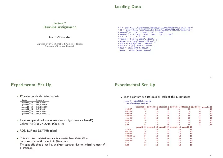
Each algorithm run 10 times on each of the 12 instances

> all <- rbind(DSJC, queen) > table(all$alg, all$inst) DSJC1000.1 DSJC1000.5 DSJC1000.9 DSJC500.1 DSJC500.5 DSJC500.9 queen11_11 010287 10 10 10 11 10 10 10 081284 10 090289 10 10 10 10 10 10 10 090289-ls 10 10 10 10 10 10 10 111085 10 10 10 10 10 10 10 DSATUR 10 10 10 10 10 10 10 RLF 10 10 10 10 10 10 10 ROS 10 10 10 10 10 10 10 queen12_12 queen13_13 queen14_14 queen15_15 queen16_16 010287 10 10 10 10 10 081284 10 10 10 10 10 090289 10 10 10 10 10 090289-ls 10 10 10 10 10 111085 10 10 10 10 10 DSATUR 10 10 10 10 10 RLF 10 10 10 10 10 ROS 10 10 10 10 10

4

slide-2
SLIDE 2

Comparative Analysis

> print(bwplot(reorder(alg, col) ~ col | inst, data = queen, layout = c(3, + 2)))

col

RLF 090289−ls 081284 111085 DSATUR ROS 090289 010287 15 20 25

  • queen11_11
  • queen12_12

15 20 25

  • queen13_13

RLF 090289−ls 081284 111085 DSATUR ROS 090289 010287

  • queen14_14

15 20 25

  • queen15_15
  • queen16_16

5

Comparative Analysis

> K <- aggregate(queen$col, list(alg = queen$alg, inst = queen$inst), + median) > print(dotplot(reorder(alg, x) ~ x | reorder(inst, x), data = K, layout = c(3, + 2), scales = list(y = list(relation = "same"))))

x

090289−ls RLF 081284 111085 DSATUR ROS 090289 010287 15 20 25

  • queen11_11
  • queen12_12

15 20 25

  • queen13_13

090289−ls RLF 081284 111085 DSATUR ROS 090289 010287

  • queen14_14

15 20 25

  • queen15_15
  • queen16_16

6

Comparative Analysis

> print(bwplot(reorder(alg, col) ~ col | reorder(inst, col), data = DSJC, + layout = c(3, 2)))

col

RLF DSATUR 090289−ls 010287 111085 090289 ROS 100 200 300

  • DSJC500.1
  • DSJC1000.1

100 200 300

  • DSJC500.5

RLF DSATUR 090289−ls 010287 111085 090289 ROS

  • DSJC1000.5

100 200 300

  • DSJC500.9
  • DSJC1000.9

7

Comparative Analysis

> print(bwplot(reorder(alg, col) ~ col | reorder(inst, col), data = DSJC, + layout = c(3, 2), col = "blue", scales = (x = list(relation = "free"))))

col

RLF DSATUR 090289−ls 010287 111085 090289 ROS 14 16 18 20

  • DSJC500.1

RLF DSATUR 090289−ls 010287 111085 090289 ROS 24 26 28 30 32

  • DSJC1000.1

RLF DSATUR 090289−ls 010287 111085 090289 ROS 60 65 70

  • DSJC500.5

RLF DSATUR 090289−ls 010287 111085 090289 ROS 110 115 120 125 130

  • DSJC1000.5

RLF DSATUR 090289−ls 010287 111085 090289 ROS 155 160 165 170 175 180

  • DSJC500.9

RLF DSATUR 090289−ls 010287 111085 090289 ROS 280 290 300 310 320 330

  • DSJC1000.9

8

slide-3
SLIDE 3

Comparative Analysis

Aggregating raw data on the random graphs

> print(bwplot(reorder(alg, col) ~ col, data = DSJC))

col

RLF DSATUR 090289−ls 010287 111085 090289 ROS 100 200 300

  • 9

Comparative Analysis

View of raw data ranked within instances and aggregated between

rank

081284 RLF DSATUR 090289−ls 111085 010287 ROS 090289 20 40 60

  • queen

20 40 60

  • DSJC

10

Trade off Solution Quality vs Run Time

> print(xyplot(time ~ col | inst, groups = alg, data = DSJC, pch = c(1:7), + scales = list(relation = "free"), auto.key = list(pch = c(1:7), + columns = 5)))

col time

5 10 15 20 25 30 24 26 28 30 32

  • DSJC1000.1

5 10 15 20 25 30 110 115 120 125 130

  • DSJC1000.5

5 10 15 20 25 30 280 290 300 310 320 330

  • DSJC1000.9

5 10 15 20 25 30 14 16 18 20

  • DSJC500.1

5 10 15 20 25 30 60 65 70

  • DSJC500.5

5 10 15 20 25 30 155 160 165 170 175 180

  • DSJC500.9

010287 081284 090289 090289−ls 111085 DSATUR RLF ROS

  • 11

Trade off Solution Quality vs Run Time

Solution quality ranked within instances Data aggregated by median value between instances

Quality Time

10^−2 10^−1 10^0 10^1 10 20 30 40 50 60 010287 090289 090289−ls 111085 DSATUR RLF ROS

DSJC

10^−3 10^−2 10^−1 10^0 10^1 10 20 30 40 50 60 70 010287 081284 090289 090289−ls 111085 DSATUR RLF ROS

queen 12

slide-4
SLIDE 4

Numerical Results

Best Solutions inst x.010287 x.081284 x.090289 x.090289-ls x.111085 x.DSATUR x.RLF x.ROS DSJC1000.1 30 31 26 29 26 24 30 DSJC1000.5 124 127 126 124 113 107 126 DSJC1000.9 317 321 321 317 297 281 315 DSJC500.1 18 20 16 18 15 14 18 DSJC500.5 71 72 63 69 64 60 72 DSJC500.9 181 175 169 174 160 155 174 queen11_11 18 14 17 13 15 15 13 16 queen12_12 20 15 20 14 16 16 14 17 queen13_13 21 16 21 16 18 17 15 19 queen14_14 23 17 23 16 19 18 17 20 queen15_15 25 18 25 18 20 19 18 21 queen16_16 27 20 25 19 22 20 19 23 Median Time (sec.) inst x.010287 x.081284 x.090289 x.090289-ls x.111085 x.DSATUR x.RLF x.ROS DSJC1000.1 1.06 0.01 9.87 30.00 0.01 0.04 0.01 DSJC1000.5 2.01 0.02 9.85 30.00 0.04 0.82 0.04 DSJC1000.9 3.02 0.02 9.87 30.00 0.07 3.98 0.06 DSJC500.1 0.74 0.00 9.91 30.00 0.00 0.01 0.00 DSJC500.5 0.99 0.01 9.87 30.00 0.01 0.12 0.01 DSJC500.9 1.25 0.01 9.77 30.00 0.02 0.54 0.02 queen11_11 0.23 30.00 0.00 9.88 30.00 0.00 0.00 0.00 queen12_12 0.27 30.00 0.00 9.88 30.00 0.00 0.00 0.00 queen13_13 0.31 30.00 0.00 9.76 30.00 0.00 0.00 0.00 queen14_14 0.36 30.00 0.00 9.82 30.00 0.00 0.00 0.00 queen15_15 0.39 30.00 0.00 9.89 30.00 0.00 0.00 0.00 queen16_16 0.49 30.00 0.00 9.71 30.00 0.00 0.00 0.00 13

DSATUR

  • 1. Let {C1, . . . , Ck}, k = |V|, be a set of empty color classes.

14

DSATUR

  • 1. Let {C1, . . . , Ck}, k = |V|, be a set of empty color classes.
  • 2. Sort vertices in decreasing order of degree and insert first into C1.

14

DSATUR

  • 1. Let {C1, . . . , Ck}, k = |V|, be a set of empty color classes.
  • 2. Sort vertices in decreasing order of degree and insert first into C1.
  • 3. Choose the next vertex to be the one with largest saturation degree, that

is, the number of differently colored adjacent vertices. (break ties preferring vertices with the maximal number of adjacent, still uncolored vertices; otherwise randomly).

14

slide-5
SLIDE 5

DSATUR

  • 1. Let {C1, . . . , Ck}, k = |V|, be a set of empty color classes.
  • 2. Sort vertices in decreasing order of degree and insert first into C1.
  • 3. Choose the next vertex to be the one with largest saturation degree, that

is, the number of differently colored adjacent vertices. (break ties preferring vertices with the maximal number of adjacent, still uncolored vertices; otherwise randomly).

  • 4. Color the vertex according to greedy heuristic.

14

DSATUR

  • 1. Let {C1, . . . , Ck}, k = |V|, be a set of empty color classes.
  • 2. Sort vertices in decreasing order of degree and insert first into C1.
  • 3. Choose the next vertex to be the one with largest saturation degree, that

is, the number of differently colored adjacent vertices. (break ties preferring vertices with the maximal number of adjacent, still uncolored vertices; otherwise randomly).

  • 4. Color the vertex according to greedy heuristic.
  • 5. If still vertices to color, goto 3. Else stop.

14

RLF

Recursive Largest First

Key idea: iteratively extract independent sets.

  • 1. Let {C1, . . . , Ck}, k = |V|, be a set of empty color classes. Set i = 1.

Let V ′ = V be a set of of still uncolored vertices.

15

RLF

Recursive Largest First

Key idea: iteratively extract independent sets.

  • 1. Let {C1, . . . , Ck}, k = |V|, be a set of empty color classes. Set i = 1.

Let V ′ = V be a set of of still uncolored vertices.

  • 2. Let U = ∅ set of vertices that cannot be added to color class Ci.

15

slide-6
SLIDE 6

RLF

Recursive Largest First

Key idea: iteratively extract independent sets.

  • 1. Let {C1, . . . , Ck}, k = |V|, be a set of empty color classes. Set i = 1.

Let V ′ = V be a set of of still uncolored vertices.

  • 2. Let U = ∅ set of vertices that cannot be added to color class Ci.
  • 3. Assign to Ci a vertex v ∈ V ′ with maximal degree in V ′

15

RLF

Recursive Largest First

Key idea: iteratively extract independent sets.

  • 1. Let {C1, . . . , Ck}, k = |V|, be a set of empty color classes. Set i = 1.

Let V ′ = V be a set of of still uncolored vertices.

  • 2. Let U = ∅ set of vertices that cannot be added to color class Ci.
  • 3. Assign to Ci a vertex v ∈ V ′ with maximal degree in V ′
  • 4. Remove from V ′ all vertices that are adjacent to v and insert them into

U.

  • 5. while V ′ is not empty:

add to Ci the vertex v′ ∈ V ′ with largest number of edges [v′, u], with u ∈ U; (break ties randomly) remove v′ from V ′ move into U all vertices in V ′ adjacent to v′.

  • 6. Set V ′ = U. If V ′ not empty i = i + 1 and goto 2. Else stop.

15