Linear Systems Linear Systems Transform Ax = b into an equivalent - - PowerPoint PPT Presentation

Linear Systems Linear Systems

Gaussian Elimination

CSE 541 Roger Crawfis

Solving Linear Systems g y

Transform Ax = b into an equivalent but Transform Ax

b into an equivalent but simpler system.

Multiply on the left by a nonsingular Multiply on the left by a nonsingular

matrix: MAx = Mb:

1 1 1 1

( ) MA Mb A M Mb A b

− − − −

Mathematically equivalent but may

1 1 1 1

( ) x MA Mb A M Mb A b = = =

Mathematically equivalent, but may

change rounding errors

Gaussian Elimination

Finding inverses of matrices is expensive Finding inverses of matrices is expensive Inverses are not necessary to solve a

linear system linear system.

Some system are much easier to solve:

Diagonal matrices Triangular matrices

Gaussian Elimination transforms the

problem into a triangular system p g y

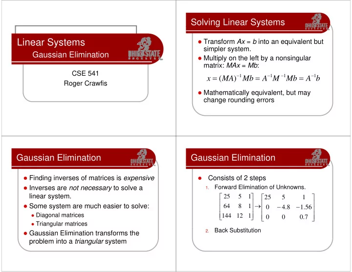
Gaussian Elimination

• Consists of 2 steps
• Consists of 2 steps

1.

Forward Elimination of Unknowns.

1 5 25 ⎤ ⎡ ⎤ ⎡ 1 5 25 56 . 1 8 . 4 1 5 25 ⎥ ⎥ ⎤ ⎢ ⎢ ⎡ − − → ⎥ ⎥ ⎥ ⎤ ⎢ ⎢ ⎢ ⎡ 1 8 64 1 5 25

B k S b tit ti

7 . ⎥ ⎥ ⎦ ⎢ ⎢ ⎣ ⎥ ⎦ ⎢ ⎣ 1 12 144

2.

Back Substitution

Gaussian Elimination

Systematically eliminate unknowns from the

equations until only a equation with only one unknown is left.

This is accomplished using three operations

p g p applied to the linear system of equations:

A given equation can be multiplied by a non-zero

constant and the result substituted for the original g equation,

A given equation can be added to a second

equation, and the result substituted for the original q g equation,

Two equations can be transposed in order.

Gaussian Elimination

Uses these elementary row operations Uses these elementary row operations

Adding a multiple of one row to another Doesn’t change the equality of the equation Doesn t change the equality of the equation

Hence the solution does not change.

The sub diagonal elements are zeroed The sub-diagonal elements are zeroed-

• ut through elementary row operations

I ifi d ( t lid )

In a specific order (next slide)

Order of Elimination

? ? ? ? ? ? ? ? ? 1 = ? ? ? 4 2 ? ? 6 5 3

Gaussian Elimination in 3D

8 3 9 4 2 2 4 2 = − + = − + z y x z y x 10 7 3 2 8 3 9 4 = + − − = + z y x z y x

Using the first equation to eliminate x

f th t t ti from the next two equations

Gaussian Elimination in 3D

4 2 2 4 2 = + = − + z y z y x 12 5 4 = + = + z y z y

Using the second equation to eliminate

f th thi d ti y from the third equation

Gaussian Elimination in 3D

4 2 2 4 2 = + = − + z y z y x 8 4 4 = = + z z y

Using the second equation to eliminate

f th thi d ti y from the third equation

Solving Triangular Systems g g y

We now have a triangular system which We now have a triangular system which

is easily solved using a technique called Backward-Substitution Backward-Substitution.

2 2 4 2 = − + z y x 8 4 4 = + z y 8 4 = z

Solving Triangular Systems g g y

If A is upper triangular we can solve If A is upper triangular, we can solve

Ax = b by:

/

n n nn n

x b A = ⎛ ⎞

1

/ , 1, ,1

n i i ij j ii j i

x b A x A i n

= +

⎛ ⎞ = − = − ⎜ ⎟ ⎝ ⎠

∑

K ⎝ ⎠

Backward Substitution

From the previous work we have From the previous work, we have

2 2 4 2 = − + z y x 2 4 = = + z z y

And substitute z in the first two equations

2 = z

And substitute z in the first two equations

Backward Substitution

4 2 2 4 4 2 = + = − + y y x 2 4 2 = = + z y

We can solve y

Backward Substitution

2 2 4 4 2 = = − + y y x 2 2 = = z y

Substitute to the first equation

Backward Substitution

2 2 4 8 2 = = − + y x 2 2 = = z y

We can solve the first equation

Backward Substitution

2 1 = − = y x 2 2 = = z y Robustness of Solution

We can measure the precision or We can measure the precision or

accuracy of our solution by calculating the residual:

Calling our computed solution x*… Calculate the distance Ax* is from b

|Ax* – b|

Some matrices are ill-conditioned

A tiny change in the input (the coefficients in

A) drastically changes the output (x*)

C# Implementation p

//convert to upper triangular form f (i t k 0 k< 1 k++) { // back substitution for (int k=0; k<n-1; k++) { try { for (int i=k+1; i<n; i++) { float s = a[i,k] / a[k,k]; b[n-1]=b[n-1] / a[n-1,n-1]; for (int i=n-2; i>=0; i--) { sum = b[i]; [ , ] [ , ]; for(int j=k+1; j<n; j++) a[i,j] -= a[k,j] * s; b[i]=b[i]-b[k] * s; } for (int j=i+1; j<n; j++) sum -= a[i,j] * x[j]; x[i] = sum / a[i,i]; } } catch (DivideByZeroException e) { }

Console.WriteLine(e.Message);

} }

Computational Complexity

Forward Elimination

p p y

For i = 1 to n-1 { // for each equation For j = i+1 to n { // for each target equation below the current

2 1 n

n

− ji

A

For k = i+1 to n { // for each element beyond pivot column

divisions

1 1

( ) 2

n i

n n i

=

− =

∑

,

ji ji ji ii

A M A A = =

}

jk jk ji ik

A A M A ← −

1 2 3

2 ( ) 3

n

n i n

−

− ≈

∑

} } }

multiply-add’s

1

3

i=

O(n3)

Computational Complexity p p y

Backward Substitution Backward Substitution

For i = n-1 to 1 { // for each equation For j = n to i+1 { // for each known variable sum = sum – Aij * xj } }

2 1 n

n

−

∑

}

multiply-add’s

1

( ) 2

i

n n i

=

− =

∑

O(n2)