
SLIDE 1
EMBnet Course – Introduction to Statistics for Biologists, Jan 2009
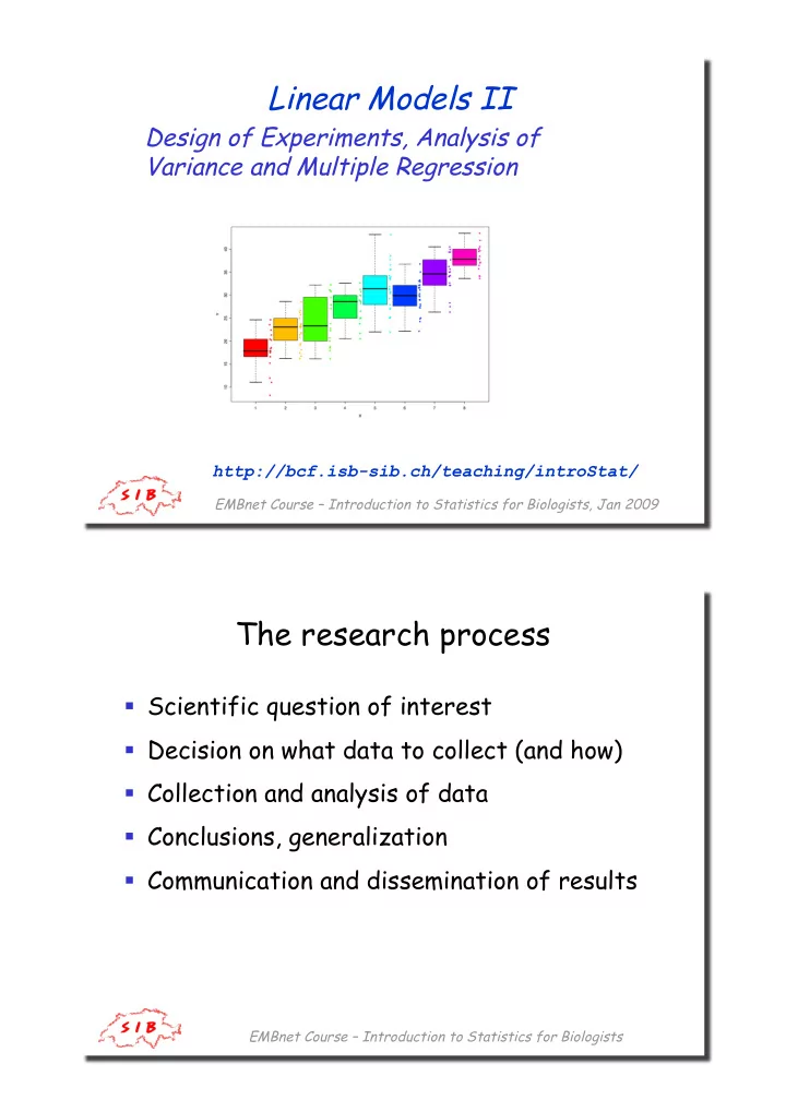
Linear Models II
http://bcf.isb-sib.ch/teaching/introStat/
Design of Experiments, Analysis of Variance and Multiple Regression
EMBnet Course – Introduction to Statistics for Biologists