Linear Approximations Suppose we want to approximate the value of a - PDF document

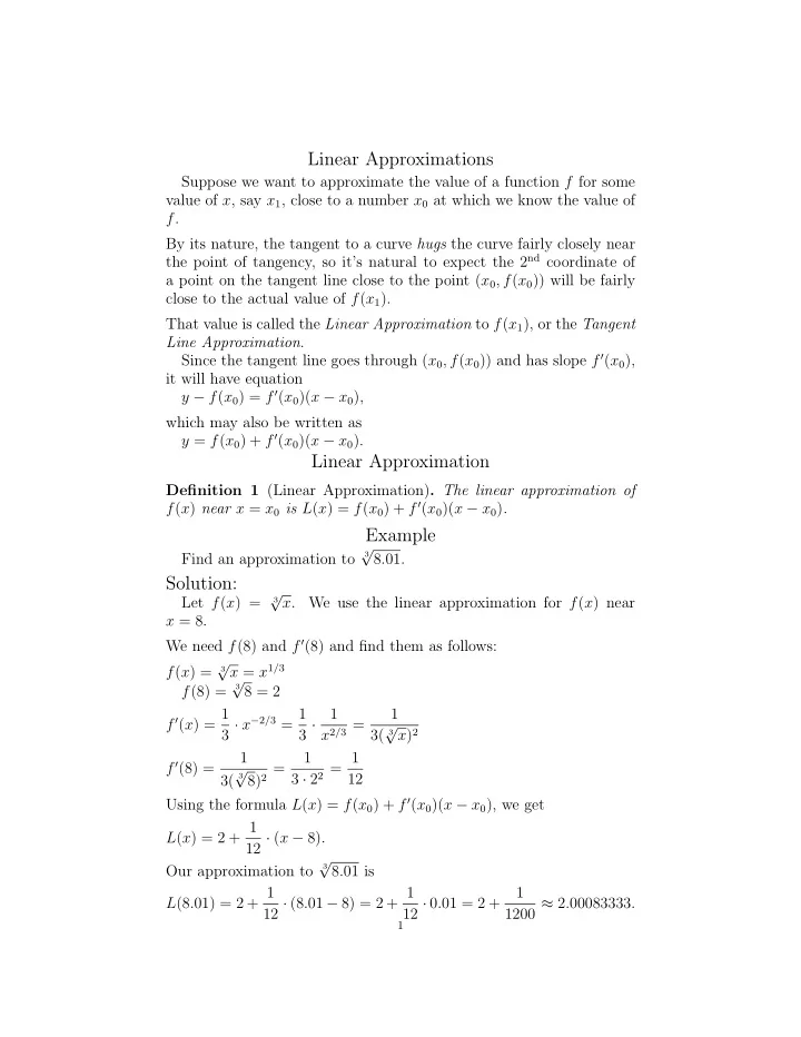
Linear Approximations Suppose we want to approximate the value of a function f for some value of x , say x 1 , close to a number x 0 at which we know the value of f . By its nature, the tangent to a curve hugs the curve fairly closely near the point of tangency, so it’s natural to expect the 2 nd coordinate of a point on the tangent line close to the point ( x 0 , f ( x 0 )) will be fairly close to the actual value of f ( x 1 ). That value is called the Linear Approximation to f ( x 1 ), or the Tangent Line Approximation . Since the tangent line goes through ( x 0 , f ( x 0 )) and has slope f ′ ( x 0 ), it will have equation y − f ( x 0 ) = f ′ ( x 0 )( x − x 0 ), which may also be written as y = f ( x 0 ) + f ′ ( x 0 )( x − x 0 ). Linear Approximation Definition 1 (Linear Approximation) . The linear approximation of f ( x ) near x = x 0 is L ( x ) = f ( x 0 ) + f ′ ( x 0 )( x − x 0 ) . Example √ Find an approximation to 3 8 . 01. Solution: √ x . Let f ( x ) = We use the linear approximation for f ( x ) near 3 x = 8. We need f (8) and f ′ (8) and find them as follows: √ x = x 1 / 3 f ( x ) = 3 √ f (8) = 3 8 = 2 f ′ ( x ) = 1 3 · x − 2 / 3 = 1 1 1 x 2 / 3 = √ x ) 2 3 · 3( 3 1 3 · 2 2 = 1 1 f ′ (8) = 8) 2 = √ 12 3 3( Using the formula L ( x ) = f ( x 0 ) + f ′ ( x 0 )( x − x 0 ), we get L ( x ) = 2 + 1 12 · ( x − 8). √ 3 Our approximation to 8 . 01 is L (8 . 01) = 2 + 1 12 · (8 . 01 − 8) = 2 + 1 1 12 · 0 . 01 = 2 + 1200 ≈ 2 . 00083333. 1

2 √ Note a calculator approximation for 3 8 . 01 is 2 . 00083299. Differentials An equivalent method of approximating values of functions is called an approximation using differentials . Definition 2 (Increment of x ) . ∆ x = x 1 − x 0 Definition 3 (Increment of y ) . ∆ y = y 1 − y 0 = f ( x 1 ) − f ( x 0 ) With this notation, f ( x 1 ) = f ( x 0 ) + ∆ y . The Linear Approximation assumes f ( x 1 ) ≈ f ( x 0 ) + f ′ ( x 0 )( x 1 − x 0 ) = f ( x 0 ) + f ′ ( x 0 )∆ x . Definition 4 (Differential of x ) . dx = ∆ x . The differential of x is synonymous with the increment of x . Definition 5 (Differential of y ) . dy = f ′ ( x 0 )∆ x = f ′ ( x 0 ) dx = dy dx · dx . With this definition, the Linear Approximation may be written f ( x 1 ) ≈ f ( x 0 ) + dy . Independently, dy may be thought of as an approximation to the amount y , or f ( x ) , changes. Example A layer of paint 0 . 001 inches thick is applied to a spherical object 16 inches in diameter. Approximately how much paint is used? Solution: The amount of paint is equal to the amount the volume of a sphere will change by if its radius increases from 8 inches to 8 . 001 inches. Letting V be the volume of the sphere and r be its radius, we know V = 4 3 πr 3 . dV dr = 4 πr 2 . Taking r 0 = 8, r 1 = 8 . 001, we find: dr = ∆ r = 8 . 001 − 8 = 0 . 001 dV r =8 = 4 π · 8 2 = 256 π � � dr

3 dV = dV dr · dr = 256 π · 0 . 001 = 0 . 256 π ≈ 0 . 8042 So it will take ≈ 0 . 256 π ≈ 0 . 8042 cubic inches of paint. Newton’s Method Newton’s Method is designed to estimate a zero of a differentiable function. It generally works faster than the Bisection Method when it works and it does not require one to first find two points at which the function has opposite signs. The drawback is that it doesn’t always work. Given a function f and an initial value x 0 , one obtains a sequence of values x 0 , x 1 , x 2 , x 3 , . . . using the formula x n = x n − 1 − f ( x n − 1 ) f ′ ( x n − 1 ) . If one is fortunate, the sequence quickly approaches a zero of f . It is generally relatively easy to set up a spreadsheet to do the calcu- lations, which can also be done using a calculator. Students familiar with any programming languages should find writing a program to im- plement Newton’s Method an easy yet educational exercise. Geometrically, x n is the first coordinate of the point at which the line tangent to the graph of f at the point ( x n − 1 , f ( x n − 1 )) crosses the x − axis. This may be seen as follows. The equation of the tangent line is y − f ( x n − 1 ) = f ′ ( x n − 1 )( x − x n − 1 ). If x n is the first coordinate of the point where this line crosses the x − axis, since the second coordinate of that point is 0, we may plug x = x n − 1 , y = 0 in that equation to get 0 − f ( x n − 1 ) = f ′ ( x n − 1 )( x n − x n − 1 ). We may then solve for x x as follows: − f ( x n − 1 ) = f ′ ( x n − 1 )( x n − x n − 1 ) − f ( x n − 1 ) f ′ ( x n − 1 ) = x n − x n − 1 x n = x n − 1 − f ( x n − 1 ) f ′ ( x n − 1 )