# Let X be a RV with E [ X ] = . Then: 2Xtu2 ) IE [ XZ - MY ] EH X ' - - PowerPoint PPT Presentation

SLIDE 1

Variance

CS 70, Summer 2019 Lecture 21, 7/30/19

1 / 26

Two Games

Game 1: Flip a coin 10 times. For each Head, you win 100. For each Tail, you lose 100. Expected Winnings on Flip i: Expected Winnings After 10 Flips:

2 / 26

fair

• Fi

Effi ]

= 100ft )

t

I

• too ) ( I )

=

I

I

ECF ]

• fi,

Effi

]

=

O

Two Games

Game 2: Flip a coin 10 times. For each Head, you win 10000. For each Tail, you lose 10000. Expected Winnings on Flip i: Expected Winnings After 10 Flips: Q: Which game would you rather play?

3 / 26

fair

• Fi

Effi

]

=

O

=

Ill

0000

)

t

I

C-

NOOO )

• Eff

7=0

Definition of Variance

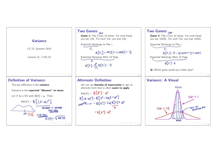
The key difference is the variance. Variance is the expected “distance” to mean. Let X be a RV with E[X] = µ. Then: Var(X) =

4 / 26

Ell

x

• ul

' I

#

Tartan

is

always

• non-neg-ttfustdD-jgxy.TW

Alternate Definition

We can use linearity of expectation to get an alternate form that is often easier to apply. Var(X) =

5 / 26

IECX

' ]

• uz

EH X

• MY ]

=

IE [ XZ

• 2µXtu2 )

linear#

=

IECXZ ]

• 2µE[ X

]tµ2

• U

= Efx

2 ]

• if

Variance: A Visual

6 / 26

• #

ftp.aais.irenrr

.

Value

SLIDE 2

Variance of a Bernoulli

Let X ∼ Bernoulli(p). Then E[X] = What is X 2? E[X 2]? Var[X] =

7 / 26

p

X'

= {

to

Wwf

Ifp

/ ENT

• tip

to

. a

• p)

=p

.

ECXZ]

• FE

EXT)

2

= F-

( pp

=

ph

• P )

X

• Bercp )

it

Ber

"

• P)

Var CX)

= rare'D

Variance of a Dice Roll

What is the variance of a single 6-sided dice roll? R = What is R2?

8 / 26

value

• f

a

dice roll

.

{ 1,2 , 3,4 , 5,63

* ÷÷÷÷

.

Variance of a Dice Roll

E[R2] = Var(R) =

9 / 26

f- ( I

t

4

t

9

t

16

t

25+36 ]

÷.ro

=

f- ( 91)

IE [ R2]

• CIEL

RIB

=

af

• EF

( Notes

.)

Variance of a Geometric

Know the variance; proof optional, but good practice with manipulating RVs. Let X ∼ Geometric(p). Strategy: Nice expression for p · E[X 2]

10 / 26

Efx

' I

=

I

. p

t

4h

• p ) p

t

9h

• ppp

t

. . .

• I
• pl Efx

Yf

• fit

p

t 4

C I

• PIP]

Subtract

from both sides

.

• PIE

=

1

• p

t

3 I I

• p ) p

t

5

C I

• PPP

t

. . . =

fz.pt/4l-plpt6CtpTpt

. . .)

t f- p

• Li
• P2P
• ftp.T

Variance of a Geometric II

From the distribution of X, we know: From E[X], we know:

11 / 26

① .€,

• lP[X=i]=pt(

I

• p

)pth

• p )2pt

. . .

• _

I IECX I

• I
• p

1-

2.

Cfp )p

• 1311
• p )2pt

. . .

②

=L

I

z

. ②

• ①

(

z.pt/4l-plpt6CtpTpt...)tfp-Ci-p7p-ltP5p.ypIEfX4=2IECX

]

• 1

ECxy=2

2

solve

for

Efxi

Variance of a Geometric III

Recall E[X] = 1

p.

12 / 26

var

CX)

• Efx 'T
• CENT)

'

• ¥

.

. ¥

• HEI

SLIDE 3

Variance of a Poisson

Same: know the variance; proof optional, but good practice with functions of RVs. Let X ∼ Poisson(λ). Strategy: Compute E[X(X − 1)].

13 / 26

IPCX

=

i ]

• Efx ( X
• 1 )]

=

l deft qf iffy

. . e- X

I i

• E) !
• E

' Fez

=

e

• xx

← taywrreen.es

j

22

=e#

I

=

A

Variance of a Poisson II

Use E[X(X − 1)] to compute Var(X).

14 / 26

var ( X)

=

Efxz ]

• Efx

])

2

=

←

→

Efxlx

• IDTECX ]
• IFECXIJ
• =

lastyszu.de

THAY

I

X

• (#

=

X

Break

Would you rather only wear sweatpants for the rest of your life, or never get to wear sweatpants ever again?

15 / 26

Properties of Variance I: Scale

Let X be a RV, and let c 2 R be a constant. Let E[X] = µ. Var(cX) =

16 / 26

e.

Var ( X) Var

C ex )

=

IE

I

• FEENY

,

lin

. =

Efe xD

• Cc EXIT

= CHECK ]

• CHE

EXT)

'

=

Cz var

( X)

Properties of Variance II: Shift

Let X be a RV, and let c 2 R be a constant. Let E[X] = µ. Then, let µ0 = E[X + c] = Var(X + c) =

17 / 26

Utc

varix )

varcxtc

)

=

Efffxtc

)

• U

'T

] =EAXtEUXY )

shift

=

'EAX

• my
• Vary ,

*

→

ten

Example: Shift It!

Consider the following RV: X =      1 w.p. 0.4 3 w.p. 0.2 5 w.p. 0.4 What is Var(X)? Shift it!

18 / 26

=

Var CX

• 3)

*of *

⇒ it

:

::

IEC X

• 351=4

. 0.8

to

.

0.2=3.2 IEC X

• 3 ]

= O

Var C C x

• 3D

=

3.2

SLIDE 4

Sum of Independent RVs

Let X1, . . . , Xn be independent RVs. Then: Var(X1 + . . . + Xn) = Var(X1) + . . . + Var(Xn) Proof: Tomorrow! Today: Focus on applications.

19 / 26

Variance of a Binomial

Let X ∼ Bin(n, p). Then, X = Here, Xi ∼ Var(X) =

20 / 26

Xitxzt

. .

.tl/nBerlp)XiiidTfdVarCX,)tVarCXz)t...tVarlXn)--n.VarCXi

)

x

• Binh

,p )

=µpFpTH

Y

• Bincnitp

)

• Vari )
• VARY )

Sum of Dependent RVs

Main strategy: linearity of expectation and indicator variables Useful Fact: (X1 + X2 + . . . + Xn)2 =

21 / 26

• 1

Xitxzt

. .

.tl/nKXitXzt.-.tXn)-=CXftXit...tXn2)tCXiXztXiX3t.-.tXn-iXn

)

• non
• D

=

Ee

,

Xi

t

jxi

alter

?

'

xix ;

HW Mixups (Fixed Points)

(In notes.) n students hand in HW. I mix up their HW randomly and return it, so that every possible mixup is equally likely. Let S = # of students who get their own HW. Last time: defined Si = Si ∼ Using linearity of expectation: E[S] =

22 / 26

indicator

for student i

getting

• wn

HW

.

Ber Hn)

ECS ,

t

Sat

. .

tsn I

= Efs , It

Elsie

. . . t ECS . ]

• = then )

HW Mixups II

Using our useful fact: E[S2] =

23 / 26

Effs

, t

Sat

. . . tsn )

' ]

= Ef En

,

sit

if jsisjl

linearity

: =

Effi ? Si 2)

t IEC

jsisj ]

=

n

. Efs

,2)

t n

In

• 1) EES , sit

÷

T HW Mixups III

What is S2

i ? E[S2 i ]?

For i 6= j, what is SiSj? E[SiSj]?

24 / 26

si

• I: If

I

* I Els it

• t

s

.sit:¥÷÷÷÷

" i ⇒

SLIDE 5

HW Mixups IV

Put it all together to compute Var(X).

25 / 26

var

C x )

• Efx 4
• CECXD

'

= FEWtncn-DEG.SI =

riff

t

n#n¥n

• I

=

• f

Summary

Today:

I Variance measures how far you deviate from

mean

I Variance is additive for independent RVs;

proof to come tomorrow

I Use linearity of expectation and indicator

variables

26 / 26