[PPT] - Lecture 9: Demand Uncertainty: Demand Uncertainty: Lecture 9: PowerPoint Presentation

SLIDE 1

Ω

Lecture 9: Lecture 9: Demand Uncertainty: Demand Uncertainty: Forecasting Forecasting

Quality Assurance in Supply Chain Management (INSE 6300/4-UU) Winter 2011

Ω

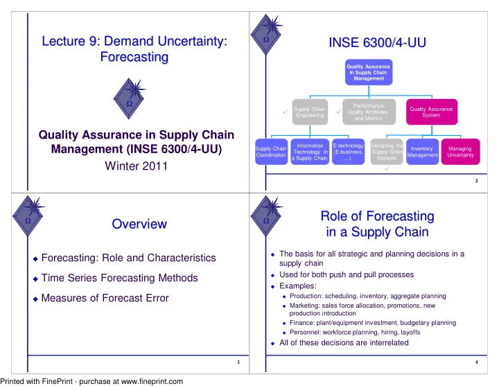
INSE 6300/4 INSE 6300/4-

UU

UU

Quality Assurance In Supply Chain Management Supply Chain Engineering Performance, Quality Attributes, and Metrics Quality Assurance System Designing the Supply Chain Network Inventory Management Supply Chain Coordination Information Technology in a Supply Chain E-technology (E-business, …) Managing Uncertainty

Ω

Overview Overview

Forecasting: Role and Characteristics Time Series Forecasting Methods Measures of Forecast Error

Ω

Role of Forecasting Role of Forecasting in a Supply Chain in a Supply Chain

The basis for all strategic and planning decisions in a

supply chain

Used for both push and pull processes Examples:

Production: scheduling, inventory, aggregate planning Marketing: sales force allocation, promotions, new

production introduction

Finance: plant/equipment investment, budgetary planning Personnel: workforce planning, hiring, layoffs

All of these decisions are interrelated

Printed with FinePrint - purchase at www.fineprint.com

SLIDE 2

Ω

Characteristics of Forecasts Characteristics of Forecasts

Forecasts are always wrong. Should

include expected value and measure of error

Long-term forecasts are less accurate

than short-term forecasts (forecast horizon is important)

Aggregate forecasts are more accurate

than disaggregate forecasts

Ω

Forecasting Methods Forecasting Methods

Qualitative: primarily subjective; rely on judgment

and opinion

Time Series: use historical demand only

Static Adaptive

Causal: use the relationship between demand

and some other factor to develop forecast

Simulation

Imitate consumer choices that give rise to demand Can combine time series and causal methods

Ω

Basic Approach to Basic Approach to Demand Forecasting Demand Forecasting

Understand the objectives of forecasting Integrate demand planning and forecasting Identify major factors that influence the demand

forecast

Understand and identify customer segments Determine the appropriate forecasting technique Establish performance and error measures for

the forecast

Ω

Components of an Components of an Observation Observation

Observed demand (O) = Systematic component (S) + Random component (R) Level (current deseasonalized demand) Trend (growth or decline in demand) Seasonality (predictable seasonal fluctuation)

Systematic component: Expected value of demand (Prediction)
Random component: The part of the forecast that deviates

from the systematic component (Estimation)

Forecast error: difference between forecast and actual demand

Printed with FinePrint - purchase at www.fineprint.com

SLIDE 3

Ω

Overview Overview

Forecasting: Role and Characteristics Time Series Forecasting Methods Measures of Forecast Error

Ω

Time Series Time Series

A time series is a sequence of data points,

measured typically at successive times, spaced at (often uniform) time intervals

Time series analysis comprises methods that

attempt to understand such time series to understand the underlying theory of the data points

Where did they come from? what generated

them?,

Time series method is used to make

forecasts (predictions)

Ω

Time Series Time Series

Time series prediction is the use of a model to predict

future events based on known past events:

To predict future data points before they are measured

Two Main Goals:

(a) identifying the nature of the phenomenon represented by

the sequence of observations,

(b) forecasting (predicting future values of the time series

variable)

Both of these goals require that the pattern of

bserved time series data is identified and more
r less formally described
Ω

Time Series Time Series

Once the pattern is established, we can interpret

and integrate it with other data (i.e., use it in the theory of the investigated phenomenon, e.g., seasonal commodity prices)

Regardless of the depth of the understanding

and the validity of the interpretation (theory) of the phenomenon, we can extrapolate the identified pattern to predict future events

Printed with FinePrint - purchase at www.fineprint.com

SLIDE 4

Ω

Time Series Patterns Time Series Patterns

Ω

Time Series Time Series Forecasting Methods Forecasting Methods

Goal is to predict systematic

component of demand

Multiplicative: (level)(trend)(seasonal

factor)

Additive: level + trend + seasonal factor Mixed: (level + trend)(seasonal factor)

Static methods Adaptive forecasting

Ω

Forecasting Methods Forecasting Methods

Static

Level, trend, and seasonality do not vary as new

demand is observed

Estimation based on historical data Using the same values for all future forecasts

Adaptive

Moving average Simple exponential smoothing Holt’s model (with trend) Winter’s model (with trend and seasonality)

Ω

Static Methods Static Methods

Assume a mixed model:

Systematic component = (level + trend)(seasonal factor) Ft+l = [L + (t + l)T]St+l forecast in period t for demand in period t + l L = estimate of level during period 0 (the deseasonalized demand) T = estimate of trend (increase or decrease in demand) St = estimate of seasonal factor for period t Dt = actual demand in period t Ft = forecast of demand in period t Printed with FinePrint - purchase at www.fineprint.com

SLIDE 5

Ω

Static Methods Static Methods

Three steps:

Estimating level and trend Estimating seasonal factors Estimating the forecast

Ω

Time Series Forecasting Time Series Forecasting

Quarter Demand Dt II, 1998 8000 III, 1998 13000 IV, 1998 23000 I, 1999 34000 II, 1999 10000 III, 1999 18000 IV, 1999 23000 I, 2000 38000 II, 2000 12000 III, 2000 13000 IV, 2000 32000 I, 2001 41000

Forecast demand for the next four quarters.

Ω

Time Series Forecasting Time Series Forecasting

10,000 20,000 30,000 40,000 50,000 9 7 , 2 9 7 , 3 9 7 , 4 9 8 , 1 9 8 , 2 9 8 , 3 9 8 , 4 9 9 , 1 9 9 , 2 9 9 , 3 9 9 , 4 , 1

Ω

Estimating Level and Trend Estimating Level and Trend

Before estimating level and trend, demand

data must be deseasonalized

Deseasonalized demand = demand that

would have been observed in the absence

f seasonal fluctuations (each season is

given equal weight)

Periodicity (p)

The number of periods after which the

seasonal cycle repeats itself

for demand at Tahoe Salt: p = 4 (average of

demand of p consecutive periods) Printed with FinePrint - purchase at www.fineprint.com

SLIDE 6

Ω

Deseasonalizing Deseasonalizing Demand Demand

[Dt-(p/2) + Dt+(p/2) + Σ 2Di] / 2p for p even

(sum is from i = t+1-(p/2) to t-1+(p/2))

Σ Di / p for p odd

(sum is from i = t-[(p-1)/2] to t+[(p-1)/2])

Dt = The average of demand from period l+1 to l+p is the deseasonalized demand for l+(p+1)/2

Ω

Deseasonalizing Deseasonalizing Demand Demand

For the example, p = 4 is even For t = 3: D3 = {D1 + D5 + Sum(i=2 to 4) [2Di]}/8 = {8000+10000+[(2)(13000)+(2)(23000)+(2)(34000)]}/8 = 19750 D4 = {D2 + D6 + Sum(i=3 to 5) [2Di]}/8 = {13000+18000+[(2)(23000)+(2)(34000)+(2)(10000)]/8 = 20625

Ω

Deseasonalizing Deseasonalizing Demand Demand

Ω

Time Series of Demand Time Series of Demand

Printed with FinePrint - purchase at www.fineprint.com

SLIDE 7

Ω

Deseasonalizing Deseasonalizing Demand Demand

Then include trend Dt = L + t T where Dt = deseasonalized demand in period t L = level (deseasonalized demand at period 0) T = trend (rate of growth of deseasonalized demand) Trend is determined by linear regression using deseasonalized demand as the dependent variable and period as the independent variable (can be done in Excel) (Tools-Data Analysis-Regression)

Ω

Linear Regression Linear Regression

linear regression is a regression method of

modeling the conditional expected value of

ne variable y given the values of some other

variable or variables x

Linear regression is called "linear" because

the relation of the response to the explanatory variables is assumed to be a linear function of some parameters

Ω

Linear Regression Linear Regression

Y = a + bX

Ω

Deseasonalizing Deseasonalizing Demand Demand

Input Y Range: C5:C12 Input X Range: A5:A12

In the example, L = 18,439 and T = 524 Printed with FinePrint - purchase at www.fineprint.com

SLIDE 8

Ω

Static Methods Static Methods

Three steps:

Estimating level and trend

Estimating seasonal factors Estimating the forecast

Ω

Estimating Seasonal Factors Estimating Seasonal Factors

Use the previous equation to calculate deseasonalized demand for each period St = Dt / Dt = seasonal factor for period t In the example, D2 = 18439 + (524)(2) = 19487 D2 = 13000 S2 = 13000/19487 = 0.67 The seasonal factors for the other periods are calculated in the same manner

Ω

Estimating Seasonal Factors Estimating Seasonal Factors

t Dt Dt-bar S-bar 1 8000 18963 0.42 = 8000/18963 2 13000 19487 0.67 = 13000/19487 3 23000 20011 1.15 = 23000/20011 4 34000 20535 1.66 = 34000/20535 5 10000 21059 0.47 = 10000/21059 6 18000 21583 0.83 = 18000/21583 7 23000 22107 1.04 = 23000/22107 8 38000 22631 1.68 = 38000/22631 9 12000 23155 0.52 = 12000/23155 10 13000 23679 0.55 = 13000/23679 11 32000 24203 1.32 = 32000/24203 12 41000 24727 1.66 = 41000/24727

Ω

Estimating Seasonal Factors Estimating Seasonal Factors

The overall seasonal factor for a “season” is then obtained by averaging all of the factors for a “season” If there are r seasonal cycles, for all periods of the form pt+i, 1<i<p, the seasonal factor for season i is Si = [Sum(j=0 to r-1) Sjp+i]/r In the example, there are 3 seasonal cycles in the data and p=4, so S1 = (0.42+0.47+0.52)/3 = 0.47 (1, 5, 9) S2 = (0.67+0.83+0.55)/3 = 0.68 (2, 6, 10) S3 = (1.15+1.04+1.32)/3 = 1.17 (3, 7, 11) S4 = (1.66+1.68+1.66)/3 = 1.67 (4, 8, 12) Printed with FinePrint - purchase at www.fineprint.com

SLIDE 9

Ω

Estimating Seasonal Factors Estimating Seasonal Factors

Ω

Estimating Seasonal Factors Estimating Seasonal Factors

Ω

Static Methods Static Methods

Three steps:

Estimating level and trend Estimating seasonal factors

Estimating the forecast

Ω

Estimating the Forecast Estimating the Forecast

Using the original equation, we can forecast the next four periods of demand: Ft+l = [L + (t + l)T]St+l F13 = (L+13T)S1 = [18439+(13)(524)](0.47) = 11868 F14 = (L+14T)S2 = [18439+(14)(524)](0.68) = 17527 F15 = (L+15T)S3 =

Printed with FinePrint - purchase at www.fineprint.com

SLIDE 10

Ω

Estimating the Forecast Estimating the Forecast

Ω

Adaptive Forecasting Adaptive Forecasting

The estimates of level, trend, and seasonality are

adjusted after each demand observation

General steps in adaptive forecasting Moving average Simple exponential smoothing Trend-corrected exponential smoothing (Holt’s

model)

Trend- and seasonality-corrected exponential

smoothing (Winter’s model)

Ω

Basic Formula for Basic Formula for Adaptive Forecasting Adaptive Forecasting

Ft+l = (Lt + lTt)St+l : forecast for period t+l in period t Lt = Estimate of level at the end of period t Tt = Estimate of trend at the end of period t St = Estimate of seasonal factor for period t Ft = Forecast of demand for period t (made period t-1 or earlier) Dt = Actual demand observed in period t Et = Forecast error in period t At = Absolute deviation for period t = |Et| MAD = Mean Absolute Deviation = average value of At

Ω

General Steps in General Steps in Adaptive Forecasting Adaptive Forecasting

1) Initialize: Compute initial estimates of level (L0), trend

(T0), and seasonal factors (S1,…,Sp). This is done as in static forecasting

2) Forecast: Forecast demand for period t+1 using the

general equation

3) Estimate error: Compute error Et+1 = Ft+1- Dt+1 4) Modify estimates: Modify the estimates of level (Lt+1),

trend (Tt+1), and seasonal factor (St+p+1), given the error Et+1 in the forecast

Repeat steps 2, 3, and 4 for each subsequent period

Printed with FinePrint - purchase at www.fineprint.com

SLIDE 11

Ω

Moving Average Moving Average

Used when demand has no observable trend or seasonality Systematic component of demand = level The level in period t is the average demand over the last N

periods (the N-period moving average)

Current forecast for all future periods is the same and is

based on the current estimate of the level Lt = (Dt + Dt-1 + … + Dt-N+1) / N Ft+1 = Lt and Ft+n = Lt After observing the demand for period t+1, revise the estimates as follows: Lt+1 = (Dt+1 + Dt + … + Dt-N+2) / N Ft+2 = Lt+1

Ω

Moving Average Example Moving Average Example

Q u a r te r D e m a n d D t II, 1 9 9 8 8 0 0 0 III, 1 9 9 8 1 3 0 0 0 IV , 1 9 9 8 2 3 0 0 0 I, 1 9 9 9 3 4 0 0 0 II, 1 9 9 9 1 0 0 0 0 III, 1 9 9 9 1 8 0 0 0 IV , 1 9 9 9 2 3 0 0 0 I, 2 0 0 0 3 8 0 0 0 II, 2 0 0 0 1 2 0 0 0 III, 2 0 0 0 1 3 0 0 0 IV , 2 0 0 0 3 2 0 0 0 I, 2 0 0 1 4 1 0 0 0

Ω

Moving Average Example Moving Average Example

From Tahoe Salt example At the end of period 4, what is the forecast demand for periods 5 through 8 using a 4-period moving average? L4 = (D4+D3+D2+D1)/4 = (34000+23000+13000+8000)/4 = 19500 F5 = 19500 = F6 = F7 = F8 Observe demand in period 5 to be D5 = 10000 Forecast error in period 5, E5 = F5 - D5 = 19500 - 10000 = 9500 Revise estimate of level in period 5: L5 = (D5+D4+D3+D2)/4 = (10000+34000+23000+13000)/4 = 20000 F6 = L5 = 20000

Ω

Printed with FinePrint - purchase at www.fineprint.com

SLIDE 12

Ω

Simple Exponential Simple Exponential Smoothing Smoothing

Whereas in Single Moving Averages the past

bservations are weighted equally,

Exponential Smoothing assigns exponentially decreasing weights as the observation get

lder

Recent observations are given relatively more

weight in forecasting than the older

bservations
Ω

Simple Exponential Simple Exponential Smoothing Smoothing

Used when demand has no observable trend or seasonality
Systematic component of demand = level
Initial estimate of level, L0, assumed to be the average of all historical data

L0 = [Sum(i=1 to n)Di]/n

Current forecast for all future periods is equal to the current estimate of the

level and is given as follows: Ft+1 = Lt and Ft+n = Lt

After observing demand Dt+1, revise the estimate of the level:

Lt+1 = αDt+1 + (1-α)Lt

What is the value of α that gives more importance to recent observations?
Compute Lt+1 using historical demand

Lt+1 = Sum(n=0 to t)[α(1-α)nDt+1-n ]

Ω

Simple Exponential Simple Exponential Smoothing Example Smoothing Example

From Tahoe Salt data, forecast demand for period 1 using exponential smoothing L0 = average of all 12 periods of data = Sum(i=1 to 12)[Di]/12 = 22083 F1 = L0 = 22083 Observed demand for period 1 = D1 = 8000 Forecast error for period 1, E1, is as follows: E1 = F1 - D1 = 22083 - 8000 = 14083 Assuming α = 0.1, revised estimate of level for period 1: L1 = αD1 + (1-α)L0 = (0.1)(8000) + (0.9)(22083) = 20675 F2 = L1 = 20675 Note that the estimate of level for period 1 is lower than in period 0

Ω

Printed with FinePrint - purchase at www.fineprint.com

SLIDE 13

Ω

Trend Trend-

Corrected Exponential

Corrected Exponential Smoothing (Holt Smoothing (Holt’ ’s Model) s Model)

Appropriate when the demand is assumed to have a level and

trend in the systematic component of demand but no seasonality

Systematic component of demand = level + trend Obtain initial estimate of level and trend by running a linear

regression of the following form:

Dt = at + b T0 = a L0 = b In period t, the forecast for future periods is expressed as follows: Ft+1 = Lt + Tt Ft+n = Lt + nTt

Ω

Trend Trend-

Corrected Exponential

Corrected Exponential Smoothing (Holt Smoothing (Holt’ ’s Model) s Model)

After observing demand for period t, revise the estimates for level and trend as follows: Lt+1 = αDt+1 + (1-α)(Lt + Tt) Tt+1 = β(Lt+1 - Lt) + (1-β)Tt α = smoothing constant for level β = smoothing constant for trend Example: Tahoe Salt demand data. Forecast demand for period 1 using Holt’s model (trend corrected exponential smoothing) Using linear regression, L0 = 12015 (linear intercept) T0 = 1549 (linear slope)

Ω

Holt Holt’ ’s Model Example s Model Example (continued) (continued)

Forecast for period 1: F1 = L0 + T0 = 12015 + 1549 = 13564 Observed demand for period 1 = D1 = 8000 E1 = F1 - D1 = 13564 - 8000 = 5564 Assume α = 0.1, β = 0.2 L1 = αD1 + (1-α)(L0+T0) = (0.1)(8000) + (0.9)(13564) = 13008 T1 = β(L1 - L0) + (1-β)T0 = (0.2)(13008 - 12015) + (0.8)(1549) = 1438 F2 = L1 + T1 = 13008 + 1438 = 14446 F5 = L1 + 4T1 = 13008 + (4)(1438) = 18760

Ω

Printed with FinePrint - purchase at www.fineprint.com

SLIDE 14

Ω

Trend Trend-

and Seasonality

and Seasonality-

Corrected Exponential

Corrected Exponential Smoothing Smoothing

Appropriate when the systematic component of demand is

assumed to have a level, trend, and seasonal factor

Systematic component = (level+trend)(seasonal factor) Assume periodicity p Obtain initial estimates of level (L0), trend (T0), seasonal

factors (S1,…,Sp) using procedure for static forecasting

In period t, the forecast for future periods is given by:

Ft+1 = (Lt+Tt)(St+1) and Ft+n = (Lt + nTt)St+n

Ω

Trend Trend-

and Seasonality

and Seasonality-

Corrected

Corrected Exponential Smoothing (continued) Exponential Smoothing (continued)

After observing demand for period t+1, revise estimates for level, trend, and seasonal factors as follows: Lt+1 = α(Dt+1/St+1) + (1-α)(Lt+Tt) Tt+1 = β(Lt+1 - Lt) + (1-β)Tt St+p+1 = γ(Dt+1/Lt+1) + (1-γ)St+1 α = smoothing constant for level β = smoothing constant for trend γ = smoothing constant for seasonal factor Example: Tahoe Salt data. Forecast demand for period 1 using Winter’s model. Initial estimates of level, trend, and seasonal factors are obtained as in the static forecasting case

Ω

Trend Trend-

and Seasonality

and Seasonality-

Corrected Exponential

Corrected Exponential Smoothing Example (continued) Smoothing Example (continued)

L0 = 18439 T0 = 524 S1=0.47, S2=0.68, S3=1.17, S4=1.67 F1 = (L0 + T0)S1 = (18439+524)(0.47) = 8913 The observed demand for period 1 = D1 = 8000 Forecast error for period 1 = E1 = F1-D1 = 8913 - 8000 = 913 Assume α = 0.1, β=0.2, γ=0.1; revise estimates for level and trend for period 1 and for seasonal factor for period 5 L1 = α(D1/S1)+(1-α)(L0+T0) = (0.1)(8000/0.47)+(0.9)(18439+524)=18769 T1 = β(L1-L0)+(1-β)T0 = (0.2)(18769-18439)+(0.8)(524) = 485 S5 = γ(D1/L1)+(1-γ)S1 = (0.1)(8000/18769)+(0.9)(0.47) = 0.47 F2 = (L1+T1)S2 = (18769 + 485)(0.68) = 13093

Ω

Printed with FinePrint - purchase at www.fineprint.com

SLIDE 15

Ω
Ω

Overview Overview

Forecasting: Role and Characteristics Time Series Forecasting Methods Measures of Forecast Error

Ω

Measures of Forecast Error Measures of Forecast Error

Forecast error = Et = Ft - Dt Mean squared error (MSE) (the variance)

MSEn = (Sum(t=1 to n)[Et

2])/n

Absolute deviation = At = |Et| Mean absolute deviation (MAD)

MADn = (Sum(t=1 to n)[At])/n σ = 1.25MAD

Ω

Measures of Forecast Error Measures of Forecast Error

Mean absolute percentage error (MAPE)

MAPEn = (Sum(t=1 to n)[|Et/ Dt|100])/n

Bias Shows whether the forecast consistently under- or

verestimates demand; should fluctuate around 0

biasn = Sum(t=1 to n)[Et]

Tracking signal Should be within the range of +6 Otherwise, possibly use a new forecasting method