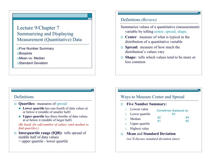
Lecture 9/Chapter 7 Summarize values of a quantitative (measurement) - PowerPoint PPT Presentation

Definitions (Review) Lecture 9/Chapter 7 Summarize values of a quantitative (measurement) variable by telling center, spread, shape. Summarizing and Displaying � Center : measure of what is typical in the Measurement (Quantitative) Data distribution of a quantitative variable � Spread: measure of how much the � Five Number Summary distribution’s values vary � Boxplots � Shape: tells which values tend to be more or � Mean vs. Median less common � Standard Deviation Definitions Ways to Measure Center and Spread � Quartiles: measures of spread: Five Number Summary: � � Lower quartile has one-fourth of data values at Lowest value 1. Sometimes displayed as or below it (middle of smaller half) Lower quartile #3 2. � Upper quartile has three-fourths of data values #2 #4 Median 3. at or below it (middle of larger half) #1 #5 Upper quartile (By hand, for odd number of values, omit median to 4. find quartiles.) Highest value 5. � Interquartile range (IQR): tells spread of Mean and Standard Deviation � middle half of data values (we’ll discuss standard deviation later) = upper quartile - lower quartile

Definition Example: 5 No. Summary, IQR, Outliers The 1.5-Times-IQR Rule identifies outliers: Background: Male earnings � 0 2 2 3 3 3 3 4 4 5 5 5 5 5 5 below lower quartile - 1.5(IQR) called low outlier � 6 6 6 6 7 8 8 10 10 12 15 20 25 42 Question: What are 5. No. Sum. & IQR? Outliers? above upper quartile +1.5(IQR) called high outlier � � Response: ___,___,___,___,___so IQR=________ � IQR IQR=__ 1.5 � IQR 1.5 � IQR 1.5 � IQR=__ 1.5 � IQR=__ Lower Upper Lower Upper quartile quartile quartile quartile High outliers Low outliers High outliers Low outliers =___ =___ above__________ below________ ( ) ( ) Displays of a Quantitative Variable Definition Displays help see the shape of the distribution. A boxplot displays median, quartiles, and � Stemplot extreme values, with special treatment for Advantage: most detail � outliers: Disadvantage: impractical for large data sets � Lower whisker to lowest non-outlier 1. � Histogram Bottom of box at lower quartile 2. Advantage: works well for any size data set � Disadvantage: some detail lost Line through box at median � 3. � Boxplot Top of box at upper quartile 4. Advantage: shows outliers, makes comparisons � Upper whisker to highest non-outlier 5. Disadvantage: much detail lost � Outliers denoted “*”.

Example: Mean vs. Median (Symmetric) Example: Constructing Boxplot Background : 29 male students’ earnings had 5 No. � Background : Heights of 10 female freshmen: � Summary: 0, 3, 5, 9, 42 and three outliers (above 18) 59 61 62 64 64 66 66 68 70 70 0 2 2 3 3 3 3 4 4 5 5 5 5 5 5 � Question: How do mean and median compare? 6 6 6 6 7 8 8 10 10 12 15 20 25 42 Question: How do we sketch boxplot? � � Response: Response: Mean = ___ � � * 40 Lower whisker to __ Median = ___ � � 30 Bottom of box at __ Mean___Median. � * Line through box at __ Note that shape is � 20 * Top of box at __ _______________ * � 10 Upper whisker to __ � Outliers marked “*” 0 Female freshmen heights (in.) Example: Mean vs. Median (Skewed) Mean vs. Median � Symmetric: � Background : Earnings ($1000) of 9 female freshmen: mean approximately equals median 1 2 2 2 3 4 7 7 17 � Skewed left / low outliers: � Question: How do mean and median compare? mean less than median � Response: � Skewed right / high outliers: Mean = ___ � mean greater than median Median = ___ � � Pronounced skewness / outliers � Mean ___Median; Report median. note that shape is � Otherwise, in general � ______________ Report mean (contains more information).

Definitions (Review) Definition/Interpretation Measures of Center � Standard deviation : square root of “average” sum of values squared distance from mean. � mean= average= number of values � median: � Mean: typical value � the middle for odd number of values � Standard deviation: typical distance of � average of middle two for even number of values values from their mean � mode: most common value Having a feel for how standard deviation measures spread is much Measures of Spread more important than being able to calculate it by hand. � Range: difference between highest & lowest � Standard deviation Example: Guessing Standard Deviation Example: Calculating a Standard Deviation Background : Female hts 59, 61, 62, 64, 64, 66, 66, 68, 70, 70 Background: Household size in U.S. has mean � � Question: What is their standard deviation? approximately 2.5 people. � Response: sq. root of “average” squared deviation from mean: � Question: Which is the standard deviation? � mean=65 (a) 0.014 (b) 0.14 (c) 1.4 (d) 14.0 deviations= ___,___,___,___,___,___,___,___,___,___ Response: ____ squared deviations= ___,___,___,___,___,___,___,___,___,___ � av sq dev=(___+___+___+___+___+___+___+___+___+___)/___ =____. Standard deviation=sq. root of “average” sq. deviation =____ (This is the typical distance from the average height 65; units are inches.)

Example: Calculating another Standard Deviation Example: Calculating another Standard Deviation Background : Female earnings 1, 2, 2, 2, 3, 4, 7, 7, 17 Response: mean=5, standard deviation=5 � � Question: What is their standard deviation? Is 5 thousand really typical for earnings? � Response: sq. root of “average” squared deviation from mean: Is 5 thousand really typical distance of earnings from average? � mean=5 Two thirds earned ___K or less; all but one were within ___K of 4 K. If the outlier 17 is omitted, mean=___, sd=___. deviations= ___,___,___,___,___,___,___,___,___ squared deviations= ___,___,___,___,___,___,___,___,___ av sq dev=(___+___+___+___+___+___+___+___+___)/_____ =_____ standard deviation=sq. root of “average” sq. deviation = ____ Is this really the typical distance from the typical earnings? The mean and, to an even greater extent, the standard deviation are distorted by outliers or skewness in a distribution. Although they are not ideal summaries for such distributions, we will see later that the normal distribution actually applies if we take a large enough sample from a non-normal population and use inference to draw conclusions about the population mean or proportion, based on our sample mean or proportion. We will begin to study the normal curve next (Chapter 8). EXTRA CREDIT (Max. 5 pts.) Summarize data for a survey variable; include mention of center, spread, and shape, and at least 2 of the 3 displays (stemplot, histogram, boxplot). Survey data is linked from my Stat 800 website www.pitt.edu/~nancyp/stat-0800/index.html and MINITAB can be used in any Pitt computer lab to produce displays and summaries. Alternatively, you can process the data by hand.