Lecture 5: Logistic Regression Feb 10 2020 Lecturer: Steven Wu - PDF document

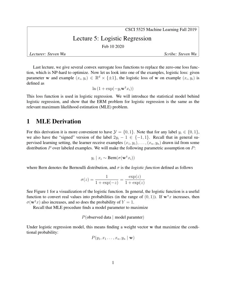
CSCI 5525 Machine Learning Fall 2019 Lecture 5: Logistic Regression Feb 10 2020 Lecturer: Steven Wu Scribe: Steven Wu Last lecture, we give several convex surrogate loss functions to replace the zero-one loss func- tion, which is NP-hard to optimize. Now let us look into one of the examples, logistic loss: given parameter w and example ( x i , y i ) ∈ R d × {± 1 } , the logistic loss of w on example ( x i , y i ) is defined as ln (1 + exp( − y i w ⊺ x i )) This loss function is used in logistic regression. We will introduce the statistical model behind logistic regression, and show that the ERM problem for logistic regression is the same as the relevant maximum likelihood estimation (MLE) problem. 1 MLE Derivation For this derivation it is more convenient to have Y = { 0 , 1 } . Note that for any label y i ∈ { 0 , 1 } , we also have the “signed” version of the label 2 y i − 1 ∈ {− 1 , 1 } . Recall that in general su- pervised learning setting, the learner receive examples ( x 1 , y 1 ) , . . . , ( x n , y n ) drawn iid from some distribution P over labeled examples. We will make the following parametric assumption on P : y i | x i ∼ Bern ( σ ( w ⊺ x i )) where Bern denotes the Bernoulli distribution, and σ is the logistic function defined as follows 1 exp( z ) σ ( z ) = 1 + exp( − z ) = 1 + exp( z ) See Figure 1 for a visualization of the logistic function. In general, the logistic function is a useful function to convert real values into probabilities (in the range of (0 , 1) ). If w ⊺ x increases, then σ ( w ⊺ x ) also increases, and so does the probability of Y = 1 . Recall that MLE procedure finds a model parameter to maximize P ( observed data | model paramter ) Under logistic regression model, this means finding a weight vector w that maximize the condi- tional probability: P ( y 1 , x 1 . . . , x n , y n | w ) 1

Figure 1: Logistic Function σ . Observe that σ ( z ) > 1 / 2 if and only if z > 0 , and σ ( z )+ σ ( − z ) = 1 . Recall in the MLE derivation for linear regression, we simplified the maximization problem as follows: w = argmax P ( y 1 , x 1 , ..., y n , x n | w ) w � n = argmax P ( y i , x i | w ) (Independence) w i =1 n � = argmax P ( y i | x i , w ) P ( x i | w ) w i =1 � n = argmax P ( y i | x i , w ) P ( x i ) ( x i is independent of w ) w i =1 n � = argmax P ( y i | x i , w ) ( P ( x i ) does not depend on w ) w i =1 This means finding a weight vector w that maximize the conditional probability (and hence the phrase maximum likelihood estimation): � n σ ( w ⊺ x i ) y i (1 − σ ( w ⊺ x i )) 1 − y i i =1 Equivalently, we would like to find the w to maximize the log likelihood: � n σ ( w ⊺ x i ) y i (1 − σ ( w ⊺ x i )) 1 − y i ln i =1 � n = ( y i ln( σ ( w ⊺ x i )) + (1 − y i ) ln(1 − σ ( w ⊺ x i ))) i =1 n � = − ( y i ln(1 + exp( − w ⊺ x i )) + (1 − y i ) ln(1 + exp( w ⊺ x i ))) (Plugging in σ ) i =1 � n = − (ln(1 + exp( − (2 y i − 1) w ⊺ x i ))) i =1 2

Note that the last step is essentially a change of variable by switching the labels to our old labels 2 y i − 1 ∈ {± 1 } . Therefore, maximizing the log-likelihood is exactly minimizing the following � n ln(1 + exp( − (2 y i − 1) w ⊺ x i )) i =1 This is exactly the ERM problem for logistic regression. Thus, the ERM problem in logistic regression is also the MLE problem under the statistical model we describe above. Solution To find the values of the parameters at minimum, we can try to find solutions for n � ∇ w ln(1 + exp( − y i w ⊺ x i )) = 0 i =1 This equation has no closed form solution, so we will use gradient descent on the negative log likelihood ℓ ( w ) = � n i =1 log(1 + exp( − y i w ⊺ x i )) . MAP Estimate Similar to the MAP estimation for linear regression, we can also have a MAP estimate for logistic regression. In the MAP estimate, we assume w is drawn from a prior belief distribution, which is often the multivariate Gaussian distribution w ∼ N ( � 0 , σ 2 I ) Our goal in MAP is to find the most likely model parameters given the data, i.e., the parameters that maximaize the posterior: P ( w | x 1 , y 1 , . . . , x n , y n ) ∝ P ( y 1 , . . . , y n | x 1 , . . . , x n , w ) P ( w ) ( ∝ means proportional to) One can show (maybe in a homework problem) that w MAP = argmax � ln ( P ( y 1 , . . . , y n | x 1 , . . . , x n , w ) P ( w )) w n � ln(1 + e − (2 y i − 1) w T � x ) + λ w ⊤ w = argmin w i =1 1 where λ = 2 σ 2 . This also corresponds to the regularized logistic regression with ℓ 2 regularization. This optimization problem also has no closed-form solutions, so we will use gradient descent to optimize the regularized loss function. 2 Multiclass Classification Now we extend these ideas to multiclass classification with Y = { 1 , . . . , K } . 3

To define a linear predictor in this setting, let us consider a linear score function f : R d → R k such that f ( x ) = W ⊺ x with a matrix W ∈ R d × K . Intuively, for each example x , the j -th coordinate of f ( x ) , denoted f ( x ) j , is a score that measures how “good” the j -th label is for this feature x . Analogously, in logistic regression w ⊺ x essentially provides a score for the label 1, and the score for label 0 is always 0. To make predictions based on the scores, we will turn score vector f ( x ) into probability distri- butions over the K labels. We will write the probability simplex over K labels as � ∆ K = { v ∈ R K ≥ 0 : p i = 1 } i In logistic regression, this is done via the logistic function. For multiclass, we can use the multino- mial logit model and define a probability vector ˆ f ( x ) ∈ ∆ K such that each coordinate j satisfies: ˆ f ( x ) j ∝ exp( f ( x ) j ) By normalization, we have exp( f ( x ) j ) ˆ f ( x ) j = � K j ′ =1 exp( f ( x ) j ′ ) Now we will define a new loss function to measure the prediction quality of ˆ f . Given two probability vectors p, q ∈ ∆ K , the cross-entropy of p and q is Cross-entropoy. � K H ( p, q ) = − p i ln q i i =1 In the special case when p = q , we have H ( p, q ) as the entropy of p , denoted H ( p ) , since � K H ( p, q ) = − p i ln q i = H ( p ) + KL ( p, q ) � �� � � �� � i =1 Entropy KL Divergence where the KL divergence term goes to 0 with p = q . To use the cross-entropy as a loss function, we need to encode the true label y i also as a probability vector. We can do that by rewriting each label y as ˜ y = e y (the standard basis vector) for any y ∈ { 1 , . . . , K } . Then given any encoded label ˜ y (from its true label y ) and real-valued score vector f ( x ) ∈ R K (along with its induced probabilistic prediction ˆ f ( x ) ∈ ∆ K ), we can 4

define the the cross-entropy loss as follows: ℓ ce (˜ y, f ( x )) = H (˜ y, ˆ y ) � � K � exp( f ( x ) j ) = − y j ln ˜ � K j =1 exp( f ( x ) j ) j =1 � � exp( f ( x ) y ) = − ln � k j =1 exp( f ( x ) j ) K � = − f ( x ) y + ln exp( f ( x ) j ) j =1 5