SLIDE 1 Lecture 3: Inversion and Chaining
Disclaimer: In this lecture, we drop the names of the judgments eph and pers, as it is clear form the context, which formula is index how. Full linear logic contains a rich set of connectives for building formulas. We have discussed the essentials in the previous lectures. For the few examples that we have seen, it seems relatively straightforward to formulate the rules, but searching for proofs is difficult. In general, there can be a lot of non-determinism, for example which rule to apply next and how to instantiate quantifiers. In this lecture we discuss how to remove some of the non-determinism, by defining to technique called inversion and chaining, which play a defining role for focusing [?]. In this presentation we follow Frank Pfenning in his lecture notes for a graduate class
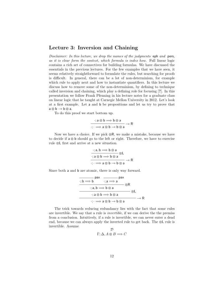
- n linear logic that he taught at Carnegie Mellon University in 2012. Let’s look
at a first example. Let a and b be propositions and let us try to prove that a ✏ b ( b ✏ a. To do this proof we start bottom up. ·; a ✏ b = ) b ✏ a ( R ·; · = ) a ✏ b ( b ✏ a Now we have a choice. If we pick ✏R, we make a mistake, because we have to decide if a ✏ b should go to the left or right. Therefore, we have to exercise rule ✏L first and arrive at a new situation. ·; a, b = ) b ✏ a ✏L ·; a ✏ b = ) b ✏ a ( R ·; · = ) a ✏ b ( b ✏ a Since both a and b are atomic, there is only way forward. pax ·; b = ) b pax ·; a = ) a ✏R ·; a, b = ) b ✏ a ✏L ·; a ✏ b = ) b ✏ a ( R ·; · = ) a ✏ b ( b ✏ a The trick towards reducing redundancy lies with the fact that some rules are invertible. We say that a rule is invertible, if we can derive the the premiss from a conclusion. Intuitively, if a rule is invertible, we can never enter a dead end, because we can always apply the inverted rule to get back. The ✏L rule is
D Γ; ∆, A ✏ B = ) C 12
SLIDE 2 Then with a clever application of cut, we just finish the derivation. ax Γ; A = ) A ax Γ; B = ) B Γ; A, B = ) A ✏ B D Γ; ∆, A ✏ B = ) C cute Γ; ∆, A, B = ) C This means that the left rule for tensor is invertible. in our example, we should always apply it if possible this rule. This raises the question, if the right rule for tensor is also applicable. Let’s try. This time, we assume that D Γ; ∆1, ∆2 = ) A ✏ B from this, we should be able to derive either premiss. Without loss of generality we aim for the left. ? ? Γ; ∆1 = ) A Since we do not know anything about the form of A, we cannot apply a right
- rule. Since we don’t know anything about Γ and ∆1, we cannot apply a left
- rule. So the only leftover candidate is the cute rule. This we can try, but then
D would have to be the left premiss, and this is not possible in the general case, as ∆1, ∆2 ⇢ ∆1. We conclude that the right rule is invertible. Here we have a connective, where the left rule is invertible, but the right rule is not. We summarize the result in form of a lemma. Lemma 8 ✏L is invertible and ✏R is not. I wonder if this special to the tensor, or perhaps is it a pattern that we can find with the other connectives? Lemma 9 ( R is invertible and ( L is not. Proof: First claim: Let D Γ; ∆ = ) A ( B Now we can show the premiss of the ( R rule as follows: D Γ; ∆ = ) A ( B ax Γ; A = ) A ax Γ; B = ) B Γ; A, A ( B = ) B cute Γ; ∆, A = ) B Let’s tend to the second claim. Assume that D Γ; ∆1, ∆2, A ( B = ) C 13
SLIDE 3
We need to show, for example, that ? ? Γ; ∆1 = ) A which is as impossible as justifying that ✏R is invertible. 2 Lemma 10 1L is invertible and 1R is not. Proof: Assume D Γ; ∆, 1 ` C It is easy to convince ourselves of the invertibility of this rule: ax Γ; · = ) 1 D Γ; ∆, 1 ` C cute Γ; ∆ ` C 2 For completeness, we’ll look the remaining two connectives, ! and 8. Lemma 11 !L is invertible and !R is not. Proof: Assume D Γ; (∆, !A) ` C It is easy to convince ourselves of the invertibility of this rule: ax (Γ, A); A = ) A copy (Γ, A); · = ) A !R (Γ, A); · = ) !A D Γ; (∆, !A) ` C cutp Γ, A; ∆ ` C !L is not invertible, although it might look at first glance that it is. 2 Lemma 12 8R is invertible and 8L is not. Proof: We only show the first claim. Assume D Γ; ∆ ` 8x : τ. A We can easily show. D Γ; ∆ ` 8x : τ. A ax Γ; A[a/x] = ) A[a/x] 8L Γ; 8x : τ. A = ) A[a/x] cute Γ, A; ∆ ` A[a/x] 8R is not invertible. 2 14
SLIDE 4 Now, after cycling through all five connectives, we notice that for some the left rules are invertible, for others the right rules. This observation al- lows us to classify formulas into two classes, ( and 8 are called negative (or asynchronous) connectives, !, 1, and✏ are called positive (or synchronous con- nectives) [?]. Nothing has been said yet about the atoms, which for now may be negative P or positive P +. Negative Formulas A, B ::= P | 8x:τ. A | A ( B Positive Formulas A+, B+ ::= P + | A ✏ B | 1 | !A Formulas A ::= A | A+ The fragment includes atomic formulas P , universal quantification 8x:τ. A, linear implication A+ ( {B+}, simultaneous conjunction A+ ✏B+ and its unit 1, the unrestricted modality !A, and an inclusion, A, of negative formulas into positive formulas. This means, that we can apply invertible rules eagerly. For a particular theorem proving goal, this might mean, applying several of those invertible rules in sequence, called an inversion phase It is interesting to note that such as phase terminates (because with every application of an invertible rule, we loose
What shall we do when we run out ouf possibilities when we do inversion? The interesting observation is that we may pick one assumption to work on and apply non-invertible rules as eagerly as possible. into so called chains. This might be surprising. It turns out, that you never have to backtrack within one
- f those chains. Either you need the entire chain to complete, or you don’t need
to work on the chosen assumption at all. This is one of the insights that is due to Andreoli [?]. To make this idea precise, we introduce a focus [A]. In our hypothetical judgment Γ; ∆ = ) A we may have at most one focus. No focus means that we are still inverting, one focus simple singles our that we are in teh middle of chain apply non-invertible rules. Not to confuse things, we write Γ; δ ! γ for this judgment, where we define δ ::= · | δ, A | δ, [A] γ ::= A | [A] First, we only consider the fragment without persistant resources. We keep 15
SLIDE 5 the Γ;, but we will consider it later. pax Γ; [P ] ! P pax+ Γ; P + ! [P +] Γ; (δ, A) ! B ( R Γ; δ ! A ( B Γ; ∆1 ! [A] Γ; ∆2, [B] ! C ( L Γ; (∆1, ∆2, [A ( B]) ! C Γ; ∆1 ! [A] Γ; ∆2 ! [B] ✏R Γ; ∆ ! [A ✏ B] Γ; (δ, A, B) ! γ ✏L Γ; (δ, A ✏ B) ! γ 1R Γ; · ! 1 Γ; δ ! C 1L Γ; (δ, 1) ! C Γ; δ ! A[a/x] 8R(a : τ) Γ; δ ! 8x:τ.A Γ; (∆, [A[t/x]]) ! C 8L, where t has sort τ Γ; (∆, [8x:τ.A]) ! C Next, we consider how to enter a chain an how to leave it. There are two rules for entering, Γ; ∆ ! [A+] focusR Γ; ∆ ! A+ Γ; ∆, [A] ! C focusL Γ; ∆, A ! C and two rules exiting (called blurring), if you read the rules bottom up. Γ; ∆ ! A blurR Γ; ∆ ! [A] Γ; ∆, A+ ! C focusL Γ; ∆, [A+] ! C In the last lecture we proved the initiality extension and the admissibility
- f the cut rule for our logic. By permitting to focus on assumptions, we need
to generalize both induction hypothesis of the admissibility theorem, by the following admissible rules. Here the admissible rules initiality expansion id Γ; A ! A idR Γ; A ! [A] idL Γ; [A] ! A Next, the addmissible cut rules. Γ; ∆ ! [A] Γ; (δ, A) ! C cutLe Γ; (∆, δ) ! C Γ; δ ! A Γ; (δ, [A]) ! C cutRe Γ; (∆, δ) ! C Γ; ∆ ! A Γ; (δ, A) ! C cutLe Γ; (∆, δ) ! C Γ; δ ! A+ Γ; (δ, A+) ! C cutRe Γ; (∆, δ) ! C 16
SLIDE 6 The main theorem is due to Andreoli, shows that focusing provability. We need to show two directions. Theorem 13 (Soundness) Let Γ; δ ! γ. If we erase all focusing brackets from δ and γ, we obtain ∆ and a formula C. Then Γ; ∆ = ) C. Proof: Easy induction. Remove focusing and bluring rules. 2 Theorem 14 (Completeness) If D Γ; ∆ = ) C then Γ; ∆ ! C. Proof: This proof is much more complicated. We show only one case that D ends in the ( L rule. D1 Γ; ∆1 = ) A D2 Γ; (∆2, B) = ) C ( L Γ; (∆1, ∆2, A ( B) = ) C By applying the induction hypothesis on D1 and D2, we obtain that Γ; ∆1 ! A and Γ; (∆2, B) ! C. We need to show that Γ; (∆1, ∆2, A ( B) ! C. Let’s start bottom up, and apply the focusing rule focusL. Γ; (∆1, ∆2, [A ( B]) ! C This can only be achieved by applying ( L, now we only need to show Γ; ∆1 ! [A] and Γ; (∆2, [B]) ! C, which looks pretty much like the result of induction hypothesis from above but not quite, because we cannot just randomly add a
- focus. We just don’t know if A is positive, and B negative. In fact, we would
make a mistake as the following counte example shows. Let ∆ = a+, a+ ( b+ and A = b+. Clearly, ·; (a+, a+ ( b+) = ) b+ is provable, in the unfocused
- system. But ·; (a+, a+ ( b+)
! b+ is not: Since b+ is not in ∆, focusing on b+ in ·; (a+, a+ ( b+) ! [b+] will fail! Instead, we will need to do some cutting. D1 Γ; ∆1 ! A idR Γ; A ! [A] idL Γ; [B] ! B ( L Γ; (A, [A ( B]) ! B focusL Γ; (A, A ( B) ! B cut Γ; (∆1, A ( B) ! B D2 Γ; (∆2, B) ! C cut Γ; (∆1, ∆2, A ( B) ! C 2 17
SLIDE 7
Finally, we address the question of persistant resources. Since last lecture, the derivability judgment refers to Γ the context of presistant resources. We will show below, that there is no need to define a focus for Γ, the only change is that when copying a resources from Γ into ∆, we will put a rule immediately into focus. As a consequence, we will introduce one new axiom rule, because if we are in right focus we must be able to look up for a positive atom in Γ without loosing right focus. This is also why the copy rule focuses only on non-positive atoms. Γ, A; ∆, [A] ` C copy, A 6= P + Γ, A; ∆ ` C pax! Γ, P +; · ! [P +] Two things until we are done. First, we need to give focused versions of the ! left and right rules. This is straightforward since we know that ! is a positive connective. Γ; · ! [A] !R Γ; · ! [!A] (Γ, A); δ ! γ !L Γ; (δ, !A) ! γ Finally, we just state that the focused version of the persistant fragment of linear logic also permits and admissible cut rule: Γ; · ! A (Γ, A); δ ! γ cut! Γ; δ ! γ
Lecture 4: Celf
In the last lecture, we will map the logic into the CLF type theory. We just motivated the following syntax for postive and negative formulas. Negative Formulas A, B ::= P | 8x:τ. A | A ( B Positive Formulas A+, B+ ::= P + | A ✏ B | 1 | !A Formulas A ::= A | A+ The first simiplicfication that we do is to commit our choices of polarities. We will not be considering positive atoms. Negative Formulas A, B ::= P | 8x:τ. A+ | A+ ( B |" A+ Positive Formulas A+, B+ ::= A+ ✏ B+ | 1 | !A |# A Now we turn formulas into types, hereby collapsing sorts and types. Neg- ative atoms turn into indexed type families. We observe a missing existential quantifier – we just add a dependent pair. It is easy to check the rules, please check this on your own. Negative Types A, B ::= P | Πx:A+. B | A+ ( B |" A+ Positive Types A+, B+ ::= 9x:A+. B+ | A+ ✏ B+ | 1 | !A |# A 18
SLIDE 8 Finally, we simplify the rules: it is suffient to restrict ourselves to either the uparrow or the downarrow. For CLF, we remove the downarrow (and use curely braces instead of the uparrow). Interestingly, the {A+} forms a monad, with which we can capture concurrency. Negative Types A, B ::= P | Πx:A+. B | A+ ( B | {A+} Positive Types A+, B+ ::= 9x:A+. B+ | A+ ✏ B+ | 1 | !A | A After all of these cosmetic changes, we need to think about objects that inhabit those types. We distinguish between three categories, normal objects N, monadic objects M, expresions E, and patterns ρ. In addition, we can make negative atoms more precise. Negative Atoms P ::= a N1 . . . Nn Negative Types A, B ::= P | Πx:A+. B | A+ ( B | {A+} Positive Types A+, B+ ::= 9x:A+. B+ | A+ ✏ B+ | 1 | !A | A where Normal Objects N ::= h N1 . . . Nn | λρ:A+.N | {E} Expressions E ::= let {ρ} = h N1 . . . Nn in E | M Monadic Objects M ::= hM1, M2i | 1 | !N |# N patterns ρ ::= hρ1, ρ2i | 1 | !x |# x One last remark. The way to program in Celf is to define a file of type family declarations and constant declartions. To help the programmer, Celf will always try to infer the types of uppercase variables and implicity Π quantifies them. That’s all for the theory folks, let’s look at the example of single transferable vote in Celf. For our specification of STV, we must introduce several predicates, which are summarized in Table 1. The uncounted-ballot, counted-ballot, hopeful, defeated, elected, quota, and winners predicates characterize the ballot box, candidates’ statuses, and the election’s state. The elect-all, defeat-min, defeat-min0, transfer, and begin predicates are used to indicate progress through the STV algorithm’s
- phases. Finally, minimum is an auxiliary predicate used in determining a can-
didate with the fewest votes. (We again assume the usual ordering predicates
- n natural numbers, such as !(N N 0).)
The linear logical axioms that specify STV are given in Fig. 2-4. Several
- f these axioms pattern-match on the shape of a list of candidates. Following
standard convention, we use [ ] to stand for the empty list and [C | L] to stand for the non-empty list with head C and tail L. (We again follow the convention that universal quantification is implicit for variables written in upper case.) These axioms faithfully encode STV in a concise and elegant fashion—rather than requiring hundreds or thousands of lines of imperative source code, our full STV specification fits on a single page! To make plain the close correspondence
- f the axioms with the natural language description of STV used in current
practice, we will now walk through their meanings. 19
SLIDE 9 Table 1: Descriptions of predicates used in the STV specification. Predicate Meaning uncounted-ballot(C, L) An uncounted ballot with highest preference for can- didate C and list L of lower preferences. counted-ballot(C, L) A ballot counted for candidate C, with list L of lower preferences. hopeful(C, N) Candidate C is not yet defeated nor elected, and N ballots have been counted for C thus far. !defeated(C) Candidate C has been (and will remain) defeated. !elected(C) Candidate C has been (and will remain) elected. !quota(Q) Q votes are needed to be elected. winners(W) The candidates in list W have been elected thus far. begin(S, H, U) Token to signal that the STV algorithm should begin
- running. There are S seats up for election, H hopeful
candidates, and U ballots cast. count-ballots(S, H, U) Token to indicate that the algorithm is counting bal- lots, and that there are S open seats, H hopeful can- didates, and U uncounted ballots remaining. !elect-all Token to indicate that there are more open seats than hopefuls remaining; all remaining hopefuls should be- come elected. defeat-min(S, H, M) Token to indicate that the algorithm is in the first step
- f determining a candidate who has the fewest votes.
There are S open seats, H hopeful candidates, and M potential minimums remaining. defeat-min0(S, H, M) Token to indicate that the algorithm is in the second step of determining a candidate who has the fewest
- votes. There are S open seats, H hopeful candidates,
and M potential minimums remaining. minimum(C, N) Candidate C’s vote count of N is a potential minimum. transfer(C, N, S, H, U) Token to indicate that newly defeated candidate C’s remaining N votes are being transferred. There are S
- pen seats, H hopeful candidates, and U uncounted
ballots. 20
SLIDE 10 Beginning the STV Algorithm. The begin/1 axiom describes the initial step of the STV algorithm: the Droop quota is computed and recorded. Ballot counting is initiated, with no candidates having been declared winners. Counting the Ballots.
- count/1 describes counting a ballot that does not cause its candidate, C,
to reach the quota: C’s vote total increases and ballot counting continues.
- count/2 describes counting a ballot that causes its candidate, C, to finally
reach the quota. C becomes elected, being a hopeful no longer, and is added to the list of winners. Any ballots remaining uncounted for C con- stitute C’s vote surplus; the surplus is randomly selected because ballots are counted in a random order. After C is elected, ballots continue to be counted.
- count/3.1, count/3.2, count/4.1, and count/4.2 express that no more bal-
lots are counted for candidates that are already either elected or defeated. The ballots transfer to the next highest preference; if none exists, the ballot is consumed—that is, the vote is wasted.
- Finally, count/5 and count/6 describe what happens when there are no
more ballots to count. If there are fewer open seats than hopefuls re- maining (count/5), then a candidate with the fewest votes is defeated; the generated defeat-min token begins this process. Otherwise, if there are at least as many open seats as hopefuls (count/6), then all remaining hopefuls are elected. Defeating a Candidate with the Fewest Votes.
- defeat-min/1 labels all hopeful candidates as potential minimums. When
there are no more hopefuls to label (i.e., when the H counter reaches 0), defeat-min/2 transitions to the second phase of defeating a candidate.
- defeat-min0/1 and defeat-min0/2 describe a random tournament for find-
ing, among the potential minimums, a candidate with the fewest votes. Candidates not selected as the minimum are restored to their hopeful sta- tus (defeat-min0/1). When only one candidate is a potential minimum (i.e., when the M counter reaches 1), that candidate must have the fewest votes; she is defeated and the process of transferring her votes begins (defeat-min0/2). Transferring a Defeated Candidate’s Votes.
- transfer/1 expresses that ballots counted for a newly defeated candidate, C,
are returned to the ballot box as uncounted ballots. As transfer/2 shows, when the N counter reaches 0, these ballots will be re-counted. Because 21
SLIDE 11 count/1 : count-ballots S H (s U) * uncounted-ballot C L * hopeful C N * !quota Q * !nat-less (s N) Q
hopeful C (s N) * count-ballots S H U}. count/2 : count-ballots (s (s S)) (s H) (s U) * uncounted-ballot C L * hopeful C N * !quota Q * !nat-lesseq Q (s N) * winners W
!elected C * winners (cons C W) * count-ballots (s S) H U}. count/3 : count-ballots (s z) H U * uncounted-ballot C L * hopeful C N * !quota Q * !nat-lesseq Q (s N) * winners W
!elected C * winners (cons C W) * !defeat-all}. count/4_1 : count-ballots S H U * uncounted-ballot C (cons C’ L) * !elected C
- o {uncounted-ballot C’ L *
count-ballots S H U}. count/4_2 : count-ballots S H U * uncounted-ballot C (cons C’ L) * !defeated C
- o {uncounted-ballot C’ L *
count-ballots S H U}. count/5_1 : count-ballots S H (s U) * uncounted-ballot C nil * !elected C
count/5_2 : count-ballots S H (s U) * uncounted-ballot C nil * !defeated C
count/6 : count-ballots S H z
Figure 2: Part 1: A linear logical specification of single transferable vote. 22
SLIDE 12 defeat-min/1 : defeat-min S (s H) M * hopeful C N
defeat-min S H (s M)}. defeat-min/2 : defeat-min S z M
defeat-min’/1 : defeat-min’ S H (s M) * minimum C N * minimum C’ N’ * !nat-less N N’
hopeful C’ N’ * defeat-min’ S (s H) M}. defeat-min’/2 : defeat-min’ S H (s z) * minimum C N
transfer C N S H z}. transfer/1 : transfer C (s N) S H U * counted-ballot C (cons C’ L)
- o {uncounted-ballot C’ L *
transfer C N S H (s U)}. transfer/2 : transfer C (s N) S H U * counted-ballot C nil
transfer/3 : transfer C z S H U * !nat-less S H
transfer/4 : transfer C z S H U * !nat-lesseq H S
defeat-all/1 : !defeat-all * hopeful C N
elect-all/1 : !elect-all * hopeful C N * winners W
winners (cons C W)}. Figure 3: Part 2: A linear logical specification of single transferable vote. 23
SLIDE 13 cleanup/1 : !defeat-all * uncounted-ballot C L
cleanup/2 : !defeat-all * counted-ballot C L
cleanup/3 : !elect-all * uncounted-ballot C L
cleanup/4 : !elect-all * counted-ballot C L
run/1 : run S H U * !nat-divmod U (s S) Q _
winners nil * count-ballots S H U}. Figure 4: Part 3: A linear logical specification of single transferable vote. 24
SLIDE 14 C is now defeated, re-counting these ballots will effectively transfer them to the next highest preference, if one exists (count/3.2 and count/4.2). Finishing the STV Election.
- elect-all/1 expresses that the STV algorithm finishes by electing all remain-
ing hopefuls. (Note that there may possibly be no remaining hopefuls at this point.) Because this is the last step of the STV algorithm, we may think of this step as continuing forever, idling once all remaining hopefuls have been elected. This justifies the use of the ! modality here and also in count/6.
- When the STV algorithm finishes, the counted ballots will remain as lin-
ear resources. The resource discipline of linear logic demands that these be used once. Therefore, the cleanup/1 axiom consumes any remaining ballots. This is safe because the STV algorithm has already filled all seats. 25