Lecture 2: Linear Regression Jan 27th 2020 Lecturer: Steven Wu - PDF document

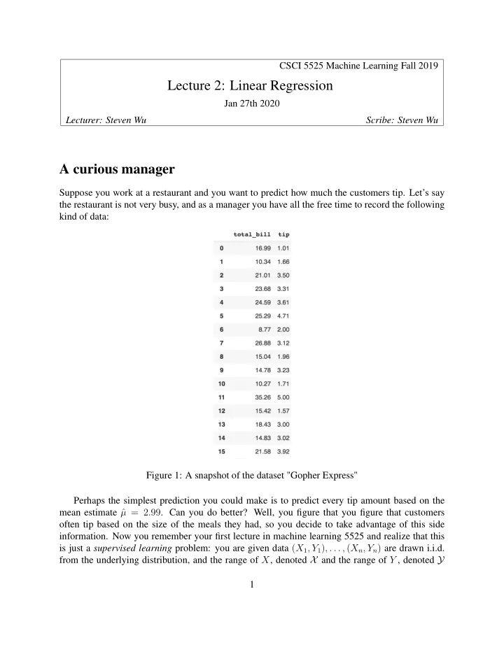
CSCI 5525 Machine Learning Fall 2019 Lecture 2: Linear Regression Jan 27th 2020 Lecturer: Steven Wu Scribe: Steven Wu A curious manager Suppose you work at a restaurant and you want to predict how much the customers tip. Let’s say the restaurant is not very busy, and as a manager you have all the free time to record the following kind of data: Figure 1: A snapshot of the dataset "Gopher Express" Perhaps the simplest prediction you could make is to predict every tip amount based on the mean estimate ˆ µ = 2 . 99 . Can you do better? Well, you figure that you figure that customers often tip based on the size of the meals they had, so you decide to take advantage of this side information. Now you remember your first lecture in machine learning 5525 and realize that this is just a supervised learning problem: you are given data ( X 1 , Y 1 ) , . . . , ( X n , Y n ) are drawn i.i.d. from the underlying distribution, and the range of X , denoted X and the range of Y , denoted Y 1

are both R . Now you would like to find a predictor/prediction function ˆ f : X → Y , so that in the future whenever you observe some new X , you can form a prediction ˆ f ( X ) . 1 Linear regression Let’s use a linear model to predict Y with an affine function : � X � ˆ f ( X ) = w ⊺ 1 � w 1 � where w = . Appending 1 makes this an affine function. To slightly abuse notation, we will w 0 � x � , and view it as the input feature. More generally, x can be in R d . just write x to denote 1 Figure 2: Fitting a affine function. But which line should we choose? 2 ERM with Least Squares Much of supervised learning follows the empirical risk minimization (ERM) approach. The general recipe of ERM takes the following steps: 2

• Pick a family of models/predictors F . (Linear models in this lecture.) • Pick a loss function ℓ . • Minimize the empirical risk over the model or equivalently the parameters. In the case of least squares regression : y = ˆ • Loss function: the least square loss for prediction ˆ f ( x ) y ) 2 ℓ ( y, ˆ y ) = ℓ ( y, ˆ y ) = ( y − ˆ Sometimes we re-scale the loss by 1 / 2 . • Goal: minimize least squares empirical risk n n f ) = 1 f ( x i )) = 1 � � R ( ˆ ˆ ℓ ( y i , ˆ ( y i − ˆ f ( x i )) 2 n n i =1 i =1 • In other words, we find a w ∈ R d (in the example d = 2 ) that minimizes ˆ R ( w ) n 1 � ( y i − w ⊺ x i ) 2 arg min n w ∈ R d i =1 We will see more examples like this, and will also learn about why ERM should work. 3 Least squares solution Let’s do some linear algebra and think about matrix forms. We can define the design matrix:   ← x ⊺ 1 → .   . A = .   ← x ⊺ n → and response vector:   y 1 .   b = . .   y n Then the empirical risk can be written as n R ( w ) = 1 ( y i − w ⊺ x i ) 2 = 1 � ˆ n � A w − b � 2 n i =1 3

Note that re-scaling the loss doesn’t change the solution, so the least squares solution is given by w ∈ R d � A w − b � 2 w ∈ arg min ˆ From calculus, we learn that a necessary condition for w to be a minimizer of ˆ R is that it needs to be a stationery point of the (re-scaled) risk function: ∇ ˆ R ( w ) = 0 This translates to the following condition ( A ⊺ A ) w − A ⊺ b = 0 or equivalently ( A ⊺ A ) w = A ⊺ b (1) Note the solutions may not be unique. Claim 3.1. The condition in equation 1 is also a sufficient condition for optimality. Proof. Let w be such that ( A ⊺ A ) w = A ⊺ b and consider any w ′ . We will show that � A w ′ − b � ≥ � A w − b � . First, note that � A w ′ − b � 2 = � A w ′ − A w + A w − b � 2 = � A w ′ − A w � 2 + 2( A w ′ − A w ) ⊺ ( A w − b ) + � A w − b � 2 Observe that ( A w ′ − A w ) ⊺ ( A w − b ) = ( w ′ − w ) ⊺ A ⊺ ( A w − b ) = ( w ′ − w ) ⊺ ( A ⊺ A w − A ⊺ b ) = 0 , where the last equality follows from the condition in (1). It follows that � A w ′ − b � 2 = � A w ′ − A w � 2 + � A w − b � 2 � �� � ≥ 0 This means any w ′ cannot have smaller loss. We can also prove the claim above with convexity. Now if we are lucky and the matrix A ⊺ A is invertible, then the least squares solution is simply the following w ∗ = ( A ⊺ A ) − 1 ( A ⊺ b ) . So how do we compute a solution for (1) when this matrix is not invertible? 4

4 SVD and Pseudoinverse We will first recall how singular value decomposition (SVD) works, and will present the thin version of SVD. Given any matrix M ∈ R m × n , we want to factorize the matrix as M = USV ⊺ , where • r is the rank of the matrix M ; • U ∈ R m × r is orthonormal, that is U ⊺ U = I r ; • V ∈ R n × r is orthonormal, that is V ⊺ V = I r ; • S ∈ R r × r is a diagonal matrix diag ( s 1 , . . . , s r ) . We could also express the factorization as a sum r � M = s i u i v ⊺ i i =1 where each u i is a column vector for U and each v i is a column vector for V . Note that { u i } spans the column space of M and { v i } spans the row space of M . This allows us to define the (Moore-Penrose) pseudoinverse r 1 � M + = v i u ⊺ i . s i i =1 Basically, we take the inverse of the singular values and reverse the positions of the v i and u i within each term. Note that if M is the full-zero matrix, then M + is also just all zeros. Now let’s return to the problem of least squares regression, where would like to fine a solution for (1). Now consider w ∗ = A + b . Claim 4.1. The vector w ∗ satisfies (1) . Proof. We can derive the following: � � � � � � r r r 1 � � � A ⊺ Aw = s i v i u ⊺ s i u i v ⊺ v i u ⊺ b (2) i i i s i i =1 i =1 i =1 � � � � r r � � = s i v i u ⊺ u i v ⊺ i v i u ⊺ b (3) i i i =1 i =1 � � � � r r � � = s i v i u ⊺ u i u ⊺ b (4) i i i =1 i =1 � � r � = s i v i u ⊺ b (5) i i =1 = A ⊺ b (6) 5

where the (4) follows because v ⊺ i v j = 0 whenever i � = j and v ⊺ i v i = 1 , and (5) follows from the fact that u ⊺ i u j = 0 whenever i � = j and u ⊺ i u i = 1 . 6