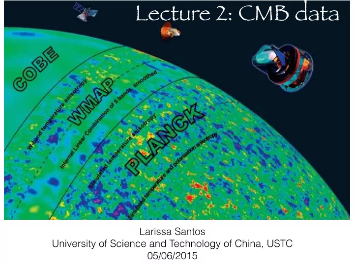
Lecture 2: CMB data Larissa Santos University of Science and - - PowerPoint PPT Presentation

Lecture 2: CMB data

Larissa Santos University of Science and Technology of China, USTC 05/06/2015

Outline

• The Interactive Data Languague
• Hierarchical Equal Area isoLatitude Pixelation
• Planck maps
• Foregrounds
• Masks
• Code for Anisotropies in the Microwave Background
• Simulations

Very short CMB timeline

SPT BOOMERANG Planck WMAP COBE

IDL

• The Interactive Data Language (IDL) is a proprietary

system distributed bu Exelis Visual Information Solution, inc

• It can be downloaded from

http://www.exelisvis.com/ProductsServices/IDL.aspx

• IDL is currently available in LINUX, Windows and

Macintosh versions

• Programming language usually used for CMB data

analysis

Screenshot

• HEALPix: Hierarchical Equal Area isoLatitude

Pixelation

• Produces a subdivision of a spherical surface in

which each pixel covers the same surface area as every other pixel

• The lowest resolution partition is comprised of 12

base pixels

• The resolution increases by 3 steps from the base

level

Gorski et al. (2005)

Definitions

• Nside
• Expresses the resolution of

the grid

• Npix
• Denotes the total number of
• pixels. Npix=12*Nside*Nside
• In the figure, the sphere is

partitioned, respectively, into 12, 48, 192 and 768 pixels (Nside = 1, 2, 4 and 8)

the ~N scaling for the non-iso-latitude sampling distributions

• Pixel numbering schemes:
• RING: counting the pixels

moving down from the north to the south pole along each iso- latitude ring.

• NESTED: arranging the pixel

indices in twelve tree structures, corresponding to base-resolution pixels

Visualization (IDL)

Planck satellite

• The Planck satellite was

launched on May14th of 2009

• The low frequency instrument

(LFI) covers 3 frequency bands

• 30, 44 and 70GHz
• The high frequency instrument

(HFI) detectors cover 6 frequency bands

• 100, 143, 217, 353, 545 and

857GHz

Planck maps

• Nside: 2048
• Npix= 5.03316e+07!!!
• Ordering: NESTED
• Format: fits file
• FITS (Flexible Image Transport System) is the data

format most widely used within astronomy for transporting, analyzing and archiving scientific data files

• They can be downloaded from

http://pla.esac.esa.int/pla/

Useful HEALPix subroutines

• MAPS: read_fits_map, read_fits_s, read_tqu,

write_fits_map, write_tqu

• Down-grading and NESTED/RING pixel reordering:

ud_grade

• Example:
• map = ‘/Users/larissasantos/Documents/Dados_Planck/'

map_ilc= "COM_CompMap_CMB-smica_2048_R1.20.fits"

• read_fits_map, map+map_ilc, smica

ud_grade, smica, a1, nside_out=8, order_in='nested', order_out='ring'

Planck frequency maps

Example of a degraded CMB map

Examples of CMB visualization

Foregrounds

• Light coming from foreground sources in our

galaxy or other galaxies must be measured accurately, so as to separate out this light from the CMB signal

Foreground overview

• Synchrotron radiation:

emission of relativistic electrons gyrating in a magnetic field

• Free-Free: emission of

electrons when deflected by massive ions

10 30 100 300 1000

Frequency (GHz)

10

• 1

10 10

1

10

2

Rms brightness temperature (µKRJ)

C M B T h e r m a l d u s t Free-free S y n c h r

• t

r

• n

30 44 70 100 143 217 353 545 857 Spinning dust

CO 1-0

Sum fg

• Thermal dust: emission from interstellar dust grains

mostly made of graphites, silicates and polycyclic aromatic hydrocarbons (PAHs)

• Spinning dust: the most plausible candidate is tiny

PAH particles spinning with dipole moment

• CO molecular clouds: Rotational transitions of

carbon monoxide

• Extragalactic point sources: some point sources

can emit in the radio-millimetric domain

The microwave sky as seen by Planck

Anisotropies of the CMB and of the cosmic infrared background Free-free (Gum nebula) Galatic dust

Planck HFI maps- CMB removed

100 GHz 857 GHz 353 GHz 143 GHz 545 GHz 217 GHz

Planck collaboration, arXiv: 1101.2048

Synchrotron emission at 23 GHz estimated in the WMAP 9-year analysis Thermal dust emission map at 353 GHz estimated by Planck experiment

α

Free-free (Dickinson et al., 2003; Finkbeiner, 2003)

Estimate map for spinning dust in the WMAP K band First estimate map for CO line emission by Planck

Noise power spectra in the HFI sky maps

• Noise power spectra on the

full sky (solid line) and after masking the Galactic plane (dotted line)

• The biggest difference is seen

for high frequency maps as expected since the Galactic signal is larger

Noise Power Spectra in the HFI Sky Maps

• Diffuse foregrounds consist of several distinct

emission processes which dominate on large angular scales

• It is important to understand the foreground

emission in order to achieve the most precise CMB maps and cosmological information

• They are os astrophysical interest and consideres

foregrounds only for CMB studies!!!

Foreground-cleaned temperature maps

• The Planck team used four methods to separate

CMB from diffuse foreground emission

• The methods can be dived in two types
• Foreground are removed by combining the

multifrequency data to minimize the variance of the CMB component

• A parameterized model of the CMB an

foreground is constructed and the CMB component is obtained by sampling from the posterior distribution of parameters

Multipole expansion: do you remember?

ΔT T θ,φ

( ) =

alm

m=−l m=l

∑

l=2 lmax

∑

Ylm θ,φ

( )

Ylm θ,φ

( ) = λlm(cosθ)eimφ

λlm x

( ) =

2l +1 4π l − m

( )!

l + m

( )!P

lm x

( )

λlm x

( ) = −1 ( )

m λl m

λlm x

( ) = 0

m ⩾ m<0 m=0

θ ∈ 0,π

[ ]

φ ∈ 0,2π

[

)

Decomposing the CMB map: quadrupole

=

• L=2

m=0 m=1,-1 m=2,-2

+ +

Octopole

L=3

= +

+ +

m=0 m=1,-1 m=2,-2 m=3,-3

HEALPix program: Anafast

• This program performs

harmonic analysis of the HEALPix maps up to a specified maximum spherical harmonic order lmax

• Anafast reads a file containing

the map and produces a file containing the temperature power spectrum and, if requested, also the polarization power spectra

• The alm coefficients computed

during the execution also can be written to a file if requested

HEALPix routine: Synfast

• This program can be used to

create HEALPix maps

• Temperature only
• Temperature and

polarization

• The map resolution, Gaussian

beam and random seed for the simulation can be selected by the user

Masks

• Even the multifrequency CMB maps are not

completely free of foregrounds

• Remove possible contaminated pixels from CMB

maps

• Planck released 3 main temperature masks with

different sky cuts and 1 polarization mask

fsky = 83.65 fsky = 78.67 fsky = 74.83

Masked CMB temperature map

CAMB Lewis Challinor and Lasenby (2000)

• Code for

Anisotropies in the Microwave Background

• CAMB Web

interface: http:// lambda.gsfc.nasa.go v/toolbox/ tb_camb_form.cfm

INPUT OUTPUT

• Cosmological parameters:

and so on h,h2Ωb,h2Ωc,h2Ωµ,Ωk,w

• CMB power spectra:
• Matter power spectrum
• Matter transfer functions

CTT ,C EE,C BB,CTE

CMB simulations

TRUE UNIV. Known only by Mother Nature Statistically realized

OBSERVABLE UNIV.

Measurements

Measured data

Analysis

Our Univ.

h

h2Ωb h2Ωc

h2Ωµ Ωk Cosmological model Interpretation What we want!!

• From the cosmological parameters

that we extract from the data we do NOT have a unique realization

• f the universe!
• Based on our cosmological model

we can generate infinitely realizations

• Each one of them generated with

the best fit parameters that we found

• For a statistical analysis compare

the realizations from your model with the measured data.

–Marcelo Gleiser

“The map of what we call reality is an ever-shifting mosaic of ideas.”