Lecture 12: Midterm Exam Review Dr. Chengjiang Long Computer - PowerPoint PPT Presentation
Lecture 12: Midterm Exam Review Dr. Chengjiang Long Computer Vision Researcher at Kitware Inc. Adjunct Professor at RPI. Email: longc3@rpi.edu Pattern recognition design cycle 2 C. Long March 6, 2018 Lecture 12 Pattern recognition design
Lecture 12: Midterm Exam Review Dr. Chengjiang Long Computer Vision Researcher at Kitware Inc. Adjunct Professor at RPI. Email: longc3@rpi.edu
Pattern recognition design cycle 2 C. Long March 6, 2018 Lecture 12
Pattern recognition design cycle Collecting training and testing data. How can we know when we have adequately large and representative set of samples? 3 C. Long March 6, 2018 Lecture 12
Training/Test Split Randomly split dataset into two parts : • Training data • Test data • Use training data to optimize parameters • Evaluate error using test data • 4 C. Long March 6, 2018 Lecture 12
Training/Test Split How many points in each set ? • Very hard question • Too few points in training set , learned classifier is bad • Too few points in test set , classifier evaluation is • insufficient Cross - validation • Leave - one - out cross - validation • 5 C. Long March 6, 2018 Lecture 12
Cross-Validation In practice • Available data = > training and validation • Train on the training data • Test on the validation data • k - fold cross validation : • Data randomly separated into k groups • Each time k • 1 groups used for training and one as testing • 6 C. Long March 6, 2018 Lecture 12
Cross Validation and Test Accuracy Using CV on training + validation • Classify test data with the best parameters from CV • 7 C. Long March 6, 2018 Lecture 12
Pattern recognition design cycle Domain dependence and prior information. Computational cost and feasibility. Discriminative features, i.e., similar values for similar patterns, and different values for different patterns. Invariant features with respect to translation, rotation and scale. Robust features with respect to occlusion, distortion, deformation, and variations in environment. 8 C. Long March 6, 2018 Lecture 12
PCA: Visualization Data points are represented in a rotated orthogonal coordinate system: the origin is the mean of the data points and the axes are provided by the eigenvectors. 9 C. Long March 6, 2018 Lecture 12
Computation of PCA In practice we compute PCA via SVD ( singular value • decomposition ) Form the centered data matrix : • [ ] = - - X ( x m ) ( x m ) p , N 1 N Compute its SVD : • = T X U D ( V ) p , p p , p N , p U and V are orthogonal matrices, D is a diagonal matrix 10 C. Long March 6, 2018 Lecture 12
Computation of PCA… Sometimes we are given only a few high dimensional data • points , i . e ., p ≥ N In such cases compute the SVD of X T : • = T T X V D ( U ) N , N N , N p , N So we get: = T X U D ( V ) p , N N , N N , N Then, proceed as before, choose only d < N significant eigenvalues for data representation: ~ = + - T x m U ( U ) ( x m ) i p , d p , d i Usually we used the features with reduced dimensions to fit the classification models. 11 C. Long March 6, 2018 Lecture 12
Fisher Linear Discriminant We need to normalize by both scatter of class 1 and • scatter of class 2 The Fisher linear discriminant is the projection on a • line in the direction v which maximizes 12 C. Long March 6, 2018 Lecture 12
Fisher Linear Discriminant Thus our objective function can be written : • Maximize J ( v ) by taking the derivative w . r . t . v and setting it to 0 • 13 C. Long March 6, 2018 Lecture 12
Fisher Linear Discriminant 14 C. Long March 6, 2018 Lecture 12
Fisher Linear Discriminant If S W has full rank ( the inverse exists ), we can convert this • to a standard eigenvalue problem But S B x for any vector x , points in the same direction as But S B x for any vector x , points in the same direction as • • μ 1 -μ 2 μ 1 -μ 2 Based on this , we can solve the eigenvalue problem • directly 15 C. Long March 6, 2018 Lecture 12
Example 16 C. Long March 6, 2018 Lecture 12
Pattern recognition design cycle How can we know how close we are to the true model underlying the patterns? Domain dependence and prior information. Definition of design criteria. Parametric vs. non-parametric models. Handling of missing features. Computational complexity. Types of models: templates, decision-theoretic or statistical,syntactic or structural, neural, and hybrid. 17 C. Long March 6, 2018 Lecture 12
The Classifiers We Have Learned So Far MLE classifier Bayesian classifiers MAP classifier Naive Bayes classifier Nonparametric classifiers KNN classifier LDF (Perceptron rule & Linear classifiers SVM classifier Minimu Square Error rule & Ho-Kashyap Procedure Kernel Tricks Nonlinear classifiers Linear classifiers Feature Mapping Φ 18 C. Long March 6, 2018 Lecture 12
Decision Rule Using Bayes’ rule : • w w p x ( / ) ( P ) ´ likelihood prior w = j j = P ( / ) x j p x ( ) evidence where = å 2 w w p x ( ) p x ( / ) ( P ) j j = j 1 Decide ω 1 if P(ω 1 /x) > P(ω 2 /x); otherwise decide ω 2 or Decide ω 1 if p(x/ω 1 )P(ω 1 )>p(x/ω 2 )P(ω 2 ); otherwise decide ω 2 or Decide ω 1 if p(x/ω 1 )/p(x/ω 2 ) >P(ω 2 )/P(ω 1 ) ; otherwise decide ω 2 19 C. Long March 6, 2018 Lecture 12
Discriminant Functions A useful way to represent a classifier is through • discriminant functions g i (x), i = 1, . . . , c, where a feature vector x is assigned to class ω i if g i ( x ) > g j ( x ) for all j i max 20 C. Long March 6, 2018 Lecture 12
Discriminants for Bayes Classifier Is the choice of g i unique ? • Replacing g i ( x ) with f ( g i ( x )), where f () is monotonically increasing , does not change the classification results . w w p ( / x ) ( P ) = i i g ( ) x i p ( ) x g i ( x )= P ( ω i / x ) = w w g ( ) x p ( / x ) ( P ) i i i = w + w g ( ) x ln p ( / x ) ln P ( ) i i i we’ll use this discriminant extensively ! 21 C. Long March 6, 2018 Lecture 12
Case 1: Statistically Independent Features with Identical Variances 22 C. Long March 6, 2018 Lecture 12
Case II: Identical Covariances Notes on Decision Boundary • As for Case I, passes through point x0 lying on the line between the two • class means. Again, x0 in the middle if priors identical Hyperplane defined by boundary generally not orthogonal to the line • between the two means 23 C. Long March 6, 2018 Lecture 12
Case III: arbitrary Nonlinear decision boundaries 24 C. Long March 6, 2018 Lecture 12
Parameter Parameter Parameter estimation Bayesian estimation / Maximum likelihood: Maximum a posteriori (MAP): values of parameters parameters as random are fixed but unknown variables having some known a priori distribution 25 C. Long March 6, 2018 Lecture 12
Maximum-Likelihood Estimation Use set of independent samples to estimate • Our goal is to determine ( value of that best • agrees with observed training data ) Note if D is fixed is not a density • 26 C. Long March 6, 2018 Lecture 12
Example: Gaussian case Assume we have c classes and • Use the information provided by the training samples • to estimate each is associated with each category. Suppose that D contains n samples, • 27 C. Long March 6, 2018 Lecture 12
Maximum-Likelihood Estimation is called the likelihood of w . r . t the set of • samples . ML estimate of is , by definition the value that • maximizes “It is the value of that best agrees with the actually observed training sample” 28 C. Long March 6, 2018 Lecture 12
Optimal Estimation Let and let be the gradient operator • We define as the log likelihood function • New problem statement : • determine that maximizes the log likelihood • 29 C. Long March 6, 2018 Lecture 12
Optimal Estimation • Local or global maximum • Local or global minimum • Saddle point • Boundary of parameter space 30 C. Long March 6, 2018 Lecture 12
Bayesian Estimation (MAP): General Theory p ( x | D ) computation can be applied to any situation in • which the unknown density can be parameterized . The basic assumptions are : • The form of is assumed known , but the value of is not known exactly Our knowledge about is assumed to be contained in a known prior density The rest of our knowledge is contained in a set D of n random variables x 1, x 2, … , xn that follows p ( x ) 31 C. Long March 6, 2018 Lecture 12
Bayesian Estimation (MAP): General Theory The basic problem is : “Compute the posterior • density ” then “Derive ” Using Bayes formula , we have : • And by the independence assumption : • 32 C. Long March 6, 2018 Lecture 12
MLE vs. MAP Maximum Likelihood estimation ( MLE ) • -- Choose value that maximizes the probability of observed data Maximum a posteriori ( MAP ) estimation • -- Choose value that is most probable given observed data and prior belief When is MAP same as MLE? 33 C. Long March 6, 2018 Lecture 12
Naïve Bayes Classifier (not BE) Simple classifier that applies Bayes ' rule with • strong ( naive ) independence assumptions A . k . a . the " independent feature model” • Often performs reasonably well despite simplicity • 34 C. Long March 6, 2018 Lecture 12
Recommend
More recommend
Explore More Topics
Stay informed with curated content and fresh updates.
