Lecture 10: Managing Lecture 10: Managing INSE 6300/4 INSE - - PowerPoint PPT Presentation

Ω

Lecture 10: Managing Lecture 10: Managing Uncertainty in the Supply Chain Uncertainty in the Supply Chain (Safety Inventory) (Safety Inventory)

Quality Assurance in Supply Chain Management (INSE 6300/4-UU) Winter 2011

• Ω

INSE 6300/4 INSE 6300/4-

• UU

UU

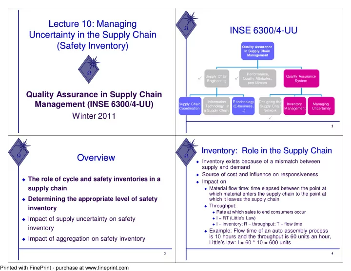
Quality Assurance In Supply Chain Management Supply Chain Engineering Performance, Quality Attributes, and Metrics Quality Assurance System Designing the Supply Chain Network Inventory Management Supply Chain Coordination Information Technology in a Supply Chain E-technology (E-business, …) Managing Uncertainty

• Ω

Overview Overview

The role of cycle and safety inventories in a

supply chain

Determining the appropriate level of safety

inventory

Impact of supply uncertainty on safety

inventory

Impact of aggregation on safety inventory

• Ω

Inventory: Role in the Supply Chain Inventory: Role in the Supply Chain

Inventory exists because of a mismatch between

supply and demand

Source of cost and influence on responsiveness Impact on Material flow time: time elapsed between the point at

which material enters the supply chain to the point at which it leaves the supply chain

Throughput: Rate at which sales to end consumers occur I = RT (Little’s Law) I = inventory; R = throughput; T = flow time Example: Flow time of an auto assembly process

is 10 hours and the throughput is 60 units an hour, Little’s law: I = 60 * 10 = 600 units Printed with FinePrint - purchase at www.fineprint.com

• Ω

Cycle Inventory Cycle Inventory

Inventory Days New shipment arrives

2 4 6 8 10 12 14 16 18 20 1 2 3 4 5 6 7 8 9 10 11 12 13 14 15 16 17 18 19 20 21

Inventory Days New shipment arrives

2 4 6 8 10 12 14 16 18 20 1 2 3 4 5 6 7 8 9 10 11 12 13 14 15 16 17 18 19 20 21

Process several flow units collectively at a given moment in time

• Ω

Role of Cycle Inventory Role of Cycle Inventory in a Supply Chain in a Supply Chain

Lot, or batch size: quantity that a supply chain stage

either produces or orders at a given time

Cycle inventory: average inventory that builds up in

the supply chain because a supply chain stage either produces or purchases in lots that are larger than those demanded by the customer

Q = lot or batch size of an order D = demand per unit time Cycle inventory = Q/2 (depends directly on lot size) Average flow time = Avg. inventory / Avg. flow rate Average flow time from cycle inventory = Q/(2D)

• Ω

Role of Cycle Inventory Role of Cycle Inventory in a Supply Chain in a Supply Chain

Q = 1000 units D = 100 units/day Cycle inventory = Q/2 = 1000/2 = 500 = Avg. inventory level from cycle inventory

• Avg. flow time = Q/2D = 1000/(2)(100) = 5 days

Cycle inventory adds 5 days to the time a unit

spends in the supply chain

Lower cycle inventory is better because:

Average flow time is lower Lower inventory holding costs

• Ω

Safety Inventory Safety Inventory

200 400 600 800 1000 1200 1 3 5 7 9 1 1 1 3 1 5 1 7 1 9 2 1 2 3 2 5 2 7 2 9 Cumulative Inflow and

• utflow

Days of the month Safety inventory Cumulative inflow Cumulative

• utflow

200 400 600 800 1000 1200 1 3 5 7 9 1 1 1 3 1 5 1 7 1 9 2 1 2 3 2 5 2 7 2 9 Cumulative Inflow and

• utflow

Days of the month Safety inventory Cumulative inflow Cumulative

• utflow

Stochastic demand: distinguishing predicted demand from the actual demand Printed with FinePrint - purchase at www.fineprint.com

• Ω

The Role of Safety Inventory The Role of Safety Inventory in a Supply Chain in a Supply Chain

Forecasts are rarely completely accurate If average demand is 1000 units per week, then half the

time actual demand will be greater than 1000, and half the time actual demand will be less than 1000; what happens when actual demand is greater than 1000?

If you kept only enough inventory in stock to satisfy

average demand, half the time you would run out

Safety inventory: Inventory carried for the purpose of

satisfying demand that exceeds the amount forecasted in a given period

• Ω

Role of Safety Inventory Role of Safety Inventory

Average inventory is therefore cycle inventory plus

safety inventory

There is a fundamental tradeoff:

Raising the level of safety inventory provides higher levels

• f product availability and customer service

Raising the level of safety inventory also raises the level of

average inventory and therefore increases holding costs

Very important in high-tech industries where

• bsolescence is a significant risk (where the value of

inventory, such as PCs, can drop in value)

• Ω

Two Questions to Answer in Two Questions to Answer in Planning Safety Inventory Planning Safety Inventory

What is the appropriate level of

safety inventory to carry?

What actions can be taken to

improve product availability while reducing safety inventory?

• Ω

Overview Overview

The role of cycle and safety inventories in a

supply chain

Determining the appropriate level of safety

inventory

Impact of supply uncertainty on safety

inventory

Impact of aggregation on safety inventory

Printed with FinePrint - purchase at www.fineprint.com

• Ω

Determining the Appropriate Determining the Appropriate Level of Safety Inventory Level of Safety Inventory

Measuring demand uncertainty Measuring product availability Replenishment policies Evaluating cycle service level and fill rate Evaluating safety level given desired cycle

service level or fill rate

Impact of required product availability and

uncertainty on safety inventory

• Ω

Determining the Appropriate Determining the Appropriate Level of Demand Uncertainty Level of Demand Uncertainty

Appropriate level of safety inventory

determined by:

Supply or demand uncertainty Desired level of product availability

Higher levels of uncertainty require higher

levels of safety inventory given a particular desired level of product availability

Higher levels of desired product availability

require higher levels of safety inventory given a particular level of uncertainty

• Ω

Measuring Demand Measuring Demand Uncertainty Uncertainty

Demand has a systematic component and a random

component

The estimate of the random component is the measure of

demand uncertainty

Random component is usually estimated by the standard

deviation of forecast error

Notation:

D = Average demand per period σD = standard deviation of demand per period (forecast error) L = lead time: time between when an order is placed and when it is received

Uncertainty of demand during lead time is what is important

• Ω

Measuring Demand Measuring Demand Uncertainty Uncertainty

Normal distribution with mean DK and std. dev. σK DK: avrg. demand during k periods = kD σK: std. dev. of demand during k periods =

σDSqrt(k)

Coefficient of variation:

cv = σ/µ = (std. dev.)/mean: size of uncertainty relative to demand Printed with FinePrint - purchase at www.fineprint.com

• Ω

Measuring Product Availability Measuring Product Availability

Product availability: a firm’s ability to fill a customer’s

• rder out of available inventory

Stockout: a customer order arrives when product is not

available

Product fill rate (fr): fraction of demand that is satisfied

from product in inventory

Order fill rate: fraction of orders that are filled from

available inventory

Cycle Service Level (CSL): fraction of replenishment

cycles that end with all customer demand met

• Ω

Replenishment Policies Replenishment Policies

Replenishment policy: decisions regarding when

to reorder and how much to reorder

Continuous review: inventory is continuously

monitored and an order of size Q is placed when the inventory level reaches the reorder point ROP

Periodic review: inventory is checked at regular

(periodic) intervals and an order is placed to raise the inventory to a specified threshold (the “order- up-to” level)

• Ω

Continuous Review Policy: Safety Continuous Review Policy: Safety Inventory and Cycle Service Level Inventory and Cycle Service Level

L: Lead time for replenishment D: Average demand per unit time σD: Standard deviation of demand per period DL: Mean demand during lead time σL: Standard deviation of demand during lead time CSL: Cycle Service Level ss:Safety inventory ROP: Reorder Point

) , , ( ) (

1

σ σ σ σ

L L L L S D L L

D D F D

ROP F CSL ss ROP CSL ss L DL = + = × = = =

−

Average Inventory = Q/2 + ss

• Ω

CSL: Cycle Service Level CSL: Cycle Service Level

CSL = Prob(demand during lead time of

L weeks ≤ ROP)

We need to obtain the distribution of

demand during the lead time

For normal distribution:

CSL = F(ROP, DL, σ L) F is the cumulative normal distribution function (F(x, µ, σ))

Printed with FinePrint - purchase at www.fineprint.com

• Ω

Example: Estimating Safety Inventory Example: Estimating Safety Inventory (Continuous Review Policy) (Continuous Review Policy)

Assume that weekly demand for palms at B&M

Computer World is normally distributed, with a mean

• f 2,500 and a standard deviation of 500

The manufacturer takes two weeks to fill an order

placed by B&M manager

The store manager currently orders 10,000 palms

when the inventory on hand drops to 6,000

Evaluate the safety inventory carried by B&M and the

average inventory carried by B&M

Evaluate the average time spend by a Palm at B&M

• Ω

Example: Estimating Safety Inventory Example: Estimating Safety Inventory (Continuous Review Policy) (Continuous Review Policy)

D = 2,500/week; σD = 500 L = 2 weeks; Q = 10,000; ROP = 6,000 DL = DL = (2500)(2) = 5000 ss = ROP - DL = 6000 - 5000 = 1000 Cycle inventory = Q/2 = 10000/2 = 5000 Average Inventory = cycle inventory + ss = 5000 + 1000 = 6000 Average Flow Time = Avg inventory / throughput = 6000/2500 = 2.4 weeks Each Palm spends an average of 2.4 weeks at B&M

• Ω

Example: Estimating Cycle Service Example: Estimating Cycle Service Level (Continuous Review Policy) Level (Continuous Review Policy)

Assume that weekly demand for palms at B&M

Computer World is normally distributed, with a mean

• f 2,500 and a standard deviation of 500

The replenishment lead time is two weeks The demand is independent from one week to the

next

Evaluate the SCL resulting from a policy of ordering

10,000 Palms when there are 6,000 Palms in inventory

• Ω

Example: Estimating Cycle Service Example: Estimating Cycle Service Level (Continuous Review Policy) Level (Continuous Review Policy)

D = 2,500/week; σD = 500 L = 2 weeks; Q = 10,000; ROP = 6,000

CSL = F(DL + ss, DL, σL) = = NORMDIST (DL + ss, DL, σL) = NORMDIST(6000,5000,707,1) = 0.92 (This value can also be determined from a Normal probability distribution table)

In 92 percent of the replenishment cycles, B&M supplies all

demand from available inventory

(500) 2 707

L D L

σ σ

= = =

Printed with FinePrint - purchase at www.fineprint.com

• Ω

Example: Estimating Cycle Service Level Example: Estimating Cycle Service Level

• Ω

Fill Rate Fill Rate

Proportion of customer

demand satisfied from stock

Stockout occurs when the

demand during lead time exceeds the reorder point

ESC is the expected shortage

per cycle (average demand in excess of reorder point in each replenishment cycle)

ss is the safety inventory Q is the order quantity

1 ( ) ( ) [1 ]

x ROP S L L S L

ESC fr Q ESC x ROP f x dx ss ESC ss ss

F f σ σ σ

∞ =

= − = −

• = −

−

• +
• ESC = -ss{1-NORMDIST(ss/σL, 0, 1, 1)} + σL NORMDIST(ss/ σL, 0, 1, 0)
• Ω

Example: Evaluating Fill Rate Example: Evaluating Fill Rate

Assume that weekly demand for palms at B&M

Computer World is normally distributed, with a mean

• f 2,500 and a standard deviation of 500

The replenishment lead time is two weeks The demand is independent from one week to the

next

Evaluate the fill rate resulting from a policy of

• rdering 10,000 Palms when there are 6,000 Palms

in inventory

• Ω

Example: Evaluating Fill Rate Example: Evaluating Fill Rate

ss = 1,000, Q = 10,000, σL = 707, Fill Rate (fr) = ? ESC = -ss{1-NORMDIST(ss/σL, 0, 1, 1)} + σL NORMDIST(ss/σL, 0, 1, 0) = -1,000{1-NORMDIST(1,000/707, 0, 1, 1)} + 707 NORMDIST(1,000/707, 0, 1, 0) = 25.13 fr = (Q - ESC)/Q = (10,000 - 25.13)/10,000 = 0.9975

Printed with FinePrint - purchase at www.fineprint.com

• Ω

Example: Evaluating Fill Rate Example: Evaluating Fill Rate

• Ω

Factors Affecting Fill Rate Factors Affecting Fill Rate

Safety inventory: Fill rate increases if

safety inventory is increased. This also increases the cycle service level

Lot size: Fill rate increases on

increasing the lot size even though cycle service level does not change

• Ω

Example: Evaluating Example: Evaluating Safety Inventory Given CSL Safety Inventory Given CSL

Weekly demand for Lego at a Wal-Mart store

is normally distributed, with a mean of 2,500 boxes and a standard deviation of 500

The replenishment lead time is two weeks Continuous review replenishment policy Evaluate the safety inventory that the store

should carry to achieve a CSL of 90 percent

• Ω

Example: Evaluating Example: Evaluating Safety Inventory Given CSL Safety Inventory Given CSL

D = 2,500/week; σD = 500 L = 2 weeks; Q = 10,000; CSL = 0.90 DL = 5000, σL = 707 (from earlier example) ss = FS-1(CSL)σL = [NORMSINV(0.90)](707) = 906 (this value can also be determined from a Normal probability distribution table) ROP = DL + ss = 5000 + 906 = 5906

Printed with FinePrint - purchase at www.fineprint.com

• Ω

Evaluating Safety Inventory Evaluating Safety Inventory Given Desired Fill Rate Given Desired Fill Rate

D = 2500, σD = 500, Q = 10000 If desired fill rate is fr = 0.975, how much safety inventory should be held? ESC = (1 - fr)Q = 250 Solve (Goal Seek: Excel)

• +
• −

− = =

• 1

250

L S L L S

ss f ss F ss ESC

• 250

1

• L

L L

ss ss ss NORMSDIST NORMDIST

• = −

− +

• Ω

Evaluating Safety Inventory Given Evaluating Safety Inventory Given Fill Rate (try different values of Fill Rate (try different values of ss ss) ) Fill Rate Safety Inventory 97.5% 67 98.0% 183 98.5% 321 99.0% 499 99.5% 767

• Ω

Impact of Required Product Availability Impact of Required Product Availability and Uncertainty on Safety Inventory and Uncertainty on Safety Inventory

Desired product availability (cycle service level or fill rate)

increases, required safety inventory increases

Demand uncertainty (σL) increases, required safety

inventory increases

Managerial levers to reduce safety inventory without

reducing product availability

reduce supplier lead time, L (better relationships with

suppliers)

reduce uncertainty in demand, σL (better forecasts,

better information collection and use)

• Ω

Overview Overview

The role of cycle and safety inventories in a

supply chain

Determining the appropriate level of safety

inventory

Impact of supply uncertainty on safety

inventory

Impact of aggregation on safety inventory

Printed with FinePrint - purchase at www.fineprint.com

• Ω

Impact of Supply Uncertainty Impact of Supply Uncertainty

D: Average demand per period σD: Standard deviation of demand per period L: Average lead time sL: Standard deviation of lead time

s D D

L D L L

L DL

2 2 2 +

= =

σ σ

• Ω

Impact of Supply Uncertainty Impact of Supply Uncertainty

D = 2,500/day; σD = 500 L = 7 days; Q = 10,000; CSL = 0.90; sL = 7 days DL = DL = (2500)(7) = 17500 ss = F-1

s(CSL)σL = NORMSINV(0.90) x 17550

= 22,491

17500 ) 7 ( ) 2500 ( 500 ) 7 (

2 2 2 2 2 2

= + = + = s D L

L

D L

σ

σ

• Ω

Impact of Supply Uncertainty Impact of Supply Uncertainty

Safety inventory when sL = 0 is 1,695 Safety inventory when sL = 1 is 3,625 Safety inventory when sL = 2 is 6,628 Safety inventory when sL = 3 is 9,760 Safety inventory when sL = 4 is 12,927 Safety inventory when sL = 5 is 16,109 Safety inventory when sL = 6 is 19,298

• Ω

Overview Overview

The role of cycle and safety inventories in a

supply chain

Determining the appropriate level of safety

inventory

Impact of supply uncertainty on safety

inventory

Impact of aggregation on safety inventory

Printed with FinePrint - purchase at www.fineprint.com

• Ω

Impact of Aggregation Impact of Aggregation

• n Safety Inventory
• n Safety Inventory

Models of aggregation Information centralization Specialization Product substitution Component commonality Postponement

• Ω

Impact of Aggregation Impact of Aggregation

σ σ σ σ σ

C L s C D C L n i i C D n i i C

CSL ss L

F D D

× = = = =

− = =

• )

(

1 1 2 1

• Ω

Example: Impact of Aggregation Example: Impact of Aggregation

A BMW dealership has 4 retail outlets serving the

entire Chicago area

Weekly demand at each outlet is normally distributed,

with a mean od D=25 cars and a std. dev. Of 5

The lead time for replenishment from the

manufacturer is 2 weeks

The correlation of demand across any pair of areas is

ρ

The dealership is considering the possibility of

replacing the 4 outlets with a single outlet (aggregate

• ption)
• Ω

Example: Impact of Aggregation Example: Impact of Aggregation

Car Dealer : 4 dealership locations (disaggregated) D = 25 cars; σD = 5 cars; L = 2 weeks; desired CSL=0.90 What would the effect be on safety stock if the 4 outlets are consolidated into 1 large outlet (aggregated)? At each disaggregated outlet: For L = 2 weeks, σL = 7.07 cars ss = Fs-1(CSL) x σL = Fs-1(0.9) x 7.07 = 9.06 Each outlet must carry 9 cars as safety stock inventory, so safety inventory for the 4 outlets in total is (4)(9) = 36 cars Printed with FinePrint - purchase at www.fineprint.com

• Ω

Example: Impact of Aggregation Example: Impact of Aggregation

One outlet (aggregated option): RC = D1 + D2 + D3 + D4 = 25+25+25+25 = 100 cars/wk σDC = Sqrt(52 + 52 + 52 + 52) = 10 σLC = σDC Sqrt(L) = (10)Sqrt(2) = (10)(1.414) = 14.14 ss = Fs-1(CSL) x σLC = Fs-1(0.9) x 14.14 =18.12

• r about 18 cars

If ρ does not equal 0 (demand is not completely independent), the impact of aggregation is not as great (Table 11.3)

• Ω

Impact of Aggregation Impact of Aggregation

If number of independent stocking locations decreases

by n, the expected level of safety inventory will be reduced by square root of n (square root law)

Many e-commerce retailers attempt to take advantage of

aggregation (Amazon) compared to bricks and mortar retailers (Borders)

Aggregation has two major disadvantages: Increase in response time to customer order Increase in transportation cost to customer Some e-commerce firms (such as Amazon) have

reduced aggregation to mitigate these disadvantages Printed with FinePrint - purchase at www.fineprint.com