Lecture 10/Chapter 8 Bell-Shaped Curves & Other Shapes From a - - PowerPoint PPT Presentation

Lecture 10/Chapter 8

Bell-Shaped Curves & Other Shapes

From a Histogram to a Frequency Curve Standard Score Using Normal Table Empirical Rule

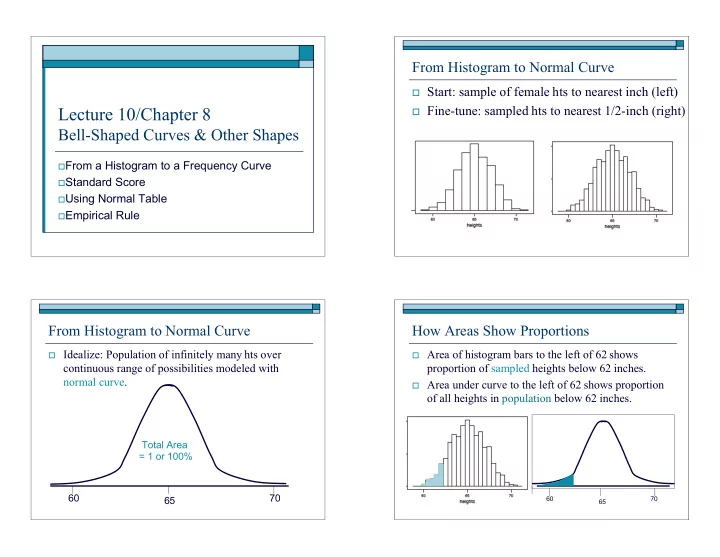
From Histogram to Normal Curve

Start: sample of female hts to nearest inch (left) Fine-tune: sampled hts to nearest 1/2-inch (right)

From Histogram to Normal Curve

Idealize: Population of infinitely many hts over

continuous range of possibilities modeled with normal curve.

65 60 70 Total Area = 1 or 100%

How Areas Show Proportions

Area of histogram bars to the left of 62 shows

proportion of sampled heights below 62 inches.

Area under curve to the left of 62 shows proportion

• f all heights in population below 62 inches.

65 60 70

Properties of Normal Curve

mean symmetric about mean bulges in the middle tapers at the ends

Background of Normal Curve

Karl Friedrich Gaus (1777-1855) was one of the first to explore normal distributions. Many distributions--such as test scores, physical characteristics, measurement errors, etc.-- naturally follow this particular pattern. If we know the shape is normal, and the value of the mean and standard deviation, we know exactly how the distribution behaves. There are infinitely many normal curves possible. Standardizing Values of Normal Distribution Put a value of a normal distribution into perspective by standardizing to its z-score:

• bserved value - mean

z = standard deviation

Example: Sign of z

Background: A person’s z-score for height is

found; its sign is negative.

Question: What do we know about the

person’s height?

Response:

Example: What z Tells Us

Background: Heights of women (in inches)

have mean 65, standard deviation 2.5. Heights

• f men have mean 70, standard deviation 3.

Question: Who is taller relative to others of

their sex: Jane at 71 inches or Joe at 76 inches?

Response: Jane has z=_________________

Joe has z=_______________

Example: More about What z Tells Us

Background: Jane’s z-score for height is +2.4

and Joe’s is +2.0.

Question: How do their heights relate to the

averages, respectively, for women and men?

Response: Jane’s height is

Joe’s height is

Example: Finding a Proportion, Given z

Background: Jane’s z-score for height is +2.4

and Joe’s is +2.0, so the proportion of women shorter than Jane is more than the proportion of men shorter than Joe.

Question: What are the proportions? Response: (See table p. 157.) The proportion

below z=+2.4 is about ____; the proportion below z=+2.0 is about ____. (Jane is in the ___th percentile; Joe is in the___th.)

Sketch #1

Example: Finding %, Given Original Value

Background: Verbal SAT scores for college-

bound students are approximately normal with mean 500, standard deviation 100.

Question: If a student scored 450, what

percentage scored less than she did?

Response: z=(value-mean)/sd =

= _____ [450 is ___ stan. deviation below mean] Table shows ____% are below this.

Sketch #2

Example: Finding Percentage Above

Background: Verbal SAT scores for college-

bound students are approximately normal with mean 500, standard deviation 100.

Question: If a student scored 400, what

percentage scored more than he did?

Response: z=(value-mean)/sd =____________

= ___ [400 is ___ stan. deviation below mean] Table shows ____% are below this so _____________% are above this.

Sketch #3

Example: Finding z, Given Percentile

Background: Verbal SAT scores for college-

bound students are approximately normal with mean 500, standard deviation 100.

Question: A student scored in the 90th

percentile; what was her score?

Response: Table shows 90th percentile has

z=____: her score is ___ sds above the mean,

• r __________________

Sketch #4

Example: Finding z, Given Percentile

Background: Verbal SAT scores for college-

bound students are approximately normal with mean 500, standard deviation 100.

Question: What is the cutoff for top 5%? Response: Proportion above = 0.05

proportion below = ____ z=_____ the value is _____stan. deviations above mean

the value is ___________________. Sketch #5

Example: Finding Proportion between Scores

Background: Verbal SAT scores for college-

bound students are approximately normal with mean 500, standard deviation 100.

Question: What proportion scored between 425

and 633?

Response: 425 has z=____; prop. below =____

633 has z=____; proportion below =_____

• Prop. with z bet.-0.75 and +1.33 is_____________

Sketch #6

Example: Proportion within 1 sd of Mean

Background: Table 8.1 p. 157 Question: What proportion of normal values

are within 1 standard deviation of the mean?

Response: Proportion below -1 is ____;

proportion below +1 is ____, so_____________ are between -1 and +1.

Sketch #7

Example: Proportion within 2 sds of Mean

Background: Table 8.1 p. 157 Question: What proportion of normal values

are within 2 standard deviations of the mean?

Response: Proportion below -2 is ______;

proportion below +2 is ____ ____________ are between -2 and +2.

Sketch #8

Example: Proportion within 3 sds of Mean

Background: Table 8.1 p. 157 Question: What proportion of normal values

are within 3 standard deviations of the mean?

Response: Proportion below -3 is_______

proportion below +3 is ______ ___________________ are between -3 and +3.

Sketch #9

Empirical Rule (68-95-99.7 Rule)

For any normal curve, approximately

68% of values are within 1 sd of mean 95% of values are within 2 sds of mean 99.7% of values are within 3 sds of mean

Example: Applying Empirical Rule

Background: IQ scores normal with mean 100,

standard deviation 15.

Question: What does Empirical Rule tell us? Response: 68% of IQ scores are between ____ and ____ 95% of IQ scores are between ____ and ____ 99.7% of IQ scores are between ____ and ____

Example: Applying Empirical Rule?

Background: Earnings for a large group of

students had mean $4000, stan. dev. $6000.

Question: What does Empirical Rule tell us? Response: 68% of earnings are between -$2000 and $10,000? 95% of earnings are between -$8000 and $16,000? 99.7% of earnings between -$14,000 and $22,000?

_________________________________________

Sketch #1 Sketch #2 Sketch #3 Sketch #4

Sketch #5 Sketch #6 Sketch #7 Sketch #8 Sketch #9 Sketch #10

Normal Practice Exercises

Try all the exercises in Lecture 11 before next class; we’ll discuss the solutions in lecture.