Lecture 03 Dynamic Programming (Chapter 15) Rod Cutting (1) Notes - - PDF document

3/44

Rod Cutting (1)

I A company has a rod of length n and wants to cut it into

smaller rods to maximize profit

I Have a table telling how much they get for rods of various

lengths: A rod of length i has price pi

I The cuts themselves are free, so profit is based solely on

the prices charged for of the rods

I If cuts only occur at integral boundaries 1, 2, . . . , n 1,

then can make or not make a cut at each of n 1 positions, so total number of possible solutions is 2n1

3/44

Notes and Questions

4/44

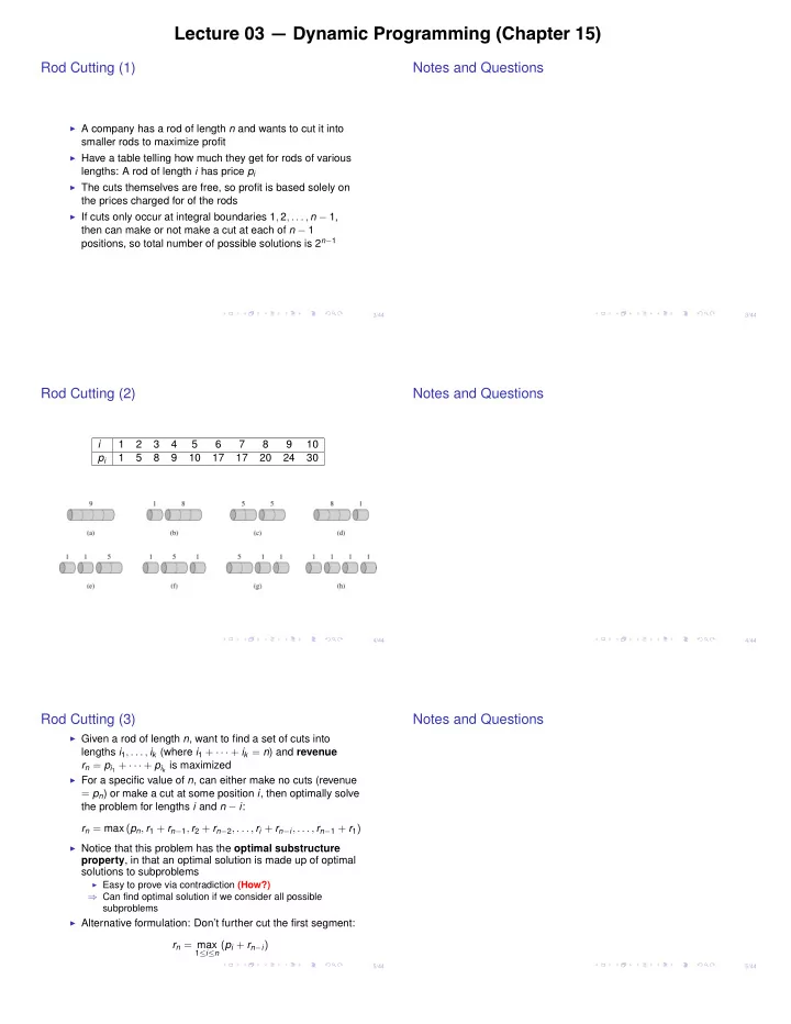
Rod Cutting (2)

i 1 2 3 4 5 6 7 8 9 10 pi 1 5 8 9 10 17 17 20 24 30

4/44

Notes and Questions

5/44

Rod Cutting (3)

I Given a rod of length n, want to find a set of cuts into

lengths i1, . . . , ik (where i1 + · · · + ik = n) and revenue rn = pi1 + · · · + pik is maximized

I For a specific value of n, can either make no cuts (revenue

= pn) or make a cut at some position i, then optimally solve the problem for lengths i and n i: rn = max (pn, r1 + rn1, r2 + rn2, . . . , ri + rni, . . . , rn1 + r1)

I Notice that this problem has the optimal substructure

property, in that an optimal solution is made up of optimal solutions to subproblems

I Easy to prove via contradiction (How?)

) Can find optimal solution if we consider all possible subproblems

I Alternative formulation: Don’t further cut the first segment:

rn = max

1in (pi + rni)

5/44

Notes and Questions

Lecture 03 — Dynamic Programming (Chapter 15)

6/44

Cut-Rod(p, n)

1 if n == 0 then 2

return 0 ;

3 q = 1 ; 4 for i = 1 to n do 5

q = max (q, p[i] + CUT-ROD(p, n i))

6 end 7 return q ;

6/44

Notes and Questions

7/44

Time Complexity

I Let T(n) be number of calls to CUT-ROD I Thus T(0) = 1 and, based on the for loop,

T(n) = 1 +

n1

X

j=0

T(j) = 2n

I Why exponential? CUT-ROD exploits the optimal

substructure property, but repeats work on these subproblems

I E.g., if the first call is for n = 4, then there will be:

I 1 call to CUT-ROD(4) I 1 call to CUT-ROD(3) I 2 calls to CUT-ROD(2) I 4 calls to CUT-ROD(1) I 8 calls to CUT-ROD(0) 7/44

Notes and Questions

8/44

Time Complexity (2)

Recursion Tree for n = 4

8/44

Notes and Questions

9/44

Dynamic Programming Algorithm

I Can save time dramatically by remembering results from

prior calls

I Two general approaches:

• 1. Top-down with memoization: Run the recursive algorithm

as defined earlier, but before recursive call, check to see if the calculation has already been done and memoized

• 2. Bottom-up: Fill in results for “small” subproblems first, then

use these to fill in table for “larger” ones

I Typically have the same asymptotic running time

9/44

Notes and Questions

10/44

Memoized-Cut-Rod-Aux(p, n, r)

1 if r[n] 0 then 2

return r[n] // r initialized to all 1 ;

3 if n == 0 then 4

q = 0 ;

5 else 6

q = 1 ;

7

for i = 1 to n do

8

q = max (q, p[i] + MEMOIZED-CUT-ROD-AUX(p, n i, r))

9

end

10

r[n] = q ;

11 return q ; 10/44

Notes and Questions

11/44

Bottom-Up-Cut-Rod(p, n)

1 Allocate r[0 . . . n] ; 2 r[0] = 0 ; 3 for j = 1 to n do 4

q = 1 ;

5

for i = 1 to j do

6

q = max (q, p[i] + r[j i])

7

end

8

r[j] = q ;

9 end 10 return r[n] ;

First solves for n = 0, then for n = 1 in terms of r[0], then for n = 2 in terms of r[0] and r[1], etc.

11/44

Notes and Questions

12/44

Example

i 1 2 3 4 5 6 7 8 9 10 pi 1 5 8 9 10 17 17 20 24 30

j = 1 i = 1 p1 + r0 = 1 = r1 j = 2 i = 1 p1 + r1 = 2 i = 2 p2 + r0 = 5 = r2 j = 3 i = 1 p1 + r2 = 1 + 5 = 6 i = 2 p2 + r1 = 5 + 1 = 6 i = 3 p3 + r0 = 8 + 0 = 8 = r3 j = 4 i = 1 p1 + r3 = 1 + 8 = 9 i = 2 p2 + r2 = 5 + 5 = 10 = r4 i = 3 p3 + r1 + 8 + 1 = 9 i = 4 p4 + r0 = 9 + 0 = 9

12/44

Notes and Questions

13/44

Time Complexity

Subproblem graph for n = 4 Both algorithms take linear time to solve for each value of n, so total time complexity is Θ(n2)

13/44

Notes and Questions

14/44

Reconstructing a Solution

I If interested in the set of cuts for an optimal solution as well

as the revenue it generates, just keep track of the choice made to optimize each subproblem

I Will add a second array s, which keeps track of the optimal

size of the first piece cut in each subproblem

14/44

Notes and Questions

15/44

Extended-Bottom-Up-Cut-Rod(p, n)

1 Allocate r[0 . . . n] and s[0 . . . n] ; 2 r[0] = 0 ; 3 for j = 1 to n do 4

q = 1 ;

5

for i = 1 to j do

6

if q < p[i] + r[j i] then

7

q = p[i] + r[j i] ;

8

s[j] = i ;

9

end

10

r[j] = q ;

11 end 12 return r, s ; 15/44

Notes and Questions

16/44

Print-Cut-Rod-Solution(p, n)

1 (r, s) = EXTENDED-BOTTOM-UP-CUT-ROD(p, n) ; 2 while n > 0 do 3

print s[n] ;

4

n = n s[n] ;

5 end

Example: i 1 2 3 4 5 6 7 8 9 10 r[i] 1 5 8 10 13 17 18 22 25 30 s[i] 1 2 3 2 2 6 1 2 3 10 If n = 10, optimal solution is no cut; if n = 7, then cut once to get segments of sizes 1 and 6

16/44

Notes and Questions

17/44

Matrix-Chain Multiplication (1)

I Given a chain of matrices hA1, . . . , Ani, goal is to compute

their product A1 · · · An

I This operation is associative, so can sequence the

multiplications in multiple ways and get the same result

I Can cause dramatic changes in number of operations

required

I Multiplying a p ⇥ q matrix by a q ⇥ r matrix requires pqr

steps and yields a p ⇥ r matrix for future multiplications

I E.g., Let A1 be 10 ⇥ 100, A2 be 100 ⇥ 5, and A3 be 5 ⇥ 50

• 1. Computing ((A1A2)A3) requires 10 · 100 · 5 = 5000 steps to

compute (A1A2) (yielding a 10 ⇥ 5), and then 10 · 5 · 50 = 2500 steps to finish, for a total of 7500

• 2. Computing (A1(A2A3)) requires 100 · 5 · 50 = 25000 steps

to compute (A2A3) (yielding a 100 ⇥ 50), and then 10 · 100 · 50 = 50000 steps to finish, for a total of 75000

17/44

Notes and Questions

18/44

Matrix-Chain Multiplication (2)

I The matrix-chain multiplication problem is to take a

chain hA1, . . . , Ani of n matrices, where matrix i has dimension pi1 ⇥ pi, and fully parenthesize the product A1 · · · An so that the number of scalar multiplications is minimized

I Brute force solution is infeasible, since its time complexity

is Ω

• 4n/n3/2

I We will follow 4-step procedure for dynamic programming:

• 1. Characterize the structure of an optimal solution
• 2. Recursively define the value of an optimal solution
• 3. Compute the value of an optimal solution
• 4. Construct an optimal solution from computed information

18/44

Notes and Questions

19/44

Step 1: Characterizing Structure of Optimal Solution

I Let Ai...j be the matrix from the product AiAi+1 · · · Aj I To compute Ai...j, must split the product and compute Ai...k

and Ak+1...j for some integer k, then multiply the two together

I Cost is the cost of computing each subproduct plus cost of

multiplying the two results

I Say that in an optimal parenthesization, the optimal split for

AiAi+1 · · · Aj is at k

I Then in an optimal solution for AiAi+1 · · · Aj, the

parenthisization of Ai · · · Ak is itself optimal for the subchain Ai · · · Ak (if not, then we could do better for the larger chain, i.e., proof by contradiction)

I Similar argument for Ak+1 · · · Aj I Thus if we make the right choice for k and then optimally

solve the subproblems recursively, we’ll end up with an

• ptimal solution

I Since we don’t know optimal k, we’ll try them all

19/44

Notes and Questions

20/44

Step 2: Recursively Defining Value of Optimal Solution

I Define m[i, j] as minimum number of scalar multiplications

needed to compute Ai...j

I (What entry in the m table will be our final answer?) I Computing m[i, j]:

• 1. If i = j, then no operations needed and m[i, i] = 0 for all i
• 2. If i < j and we split at k, then optimal number of operations

needed is the optimal number for computing Ai...k and Ak+1...j, plus the number to multiply them: m[i, j] = m[i, k] + m[k + 1, j] + pi1pkpj

• 3. Since we don’t know k, we’ll try all possible values:

m[i, j] = ⇢ 0 if i = j minik<j{m[i, k] + m[k + 1, j] + pi1pkpj} if i < j

I To track the optimal solution itself, define s[i, j] to be the

value of k used at each split

20/44

Notes and Questions

21/44

Step 3: Computing Value of Optimal Solution

I As with the rod cutting problem, many of the subproblems

we’ve defined will overlap

I Exploiting overlap allows us to solve only Θ(n2) problems

(one problem for each (i, j) pair), as opposed to exponential

I We’ll do a bottom-up implementation, based on chain

length

I Chains of length 1 are trivially solved (m[i, i] = 0 for all i) I Then solve chains of length 2, 3, etc., up to length n I Linear time to solve each problem, quadratic number of

problems, yields O(n3) total time

21/44

Notes and Questions

22/44

Matrix-Chain-Order(p, n)

1 allocate m[1 . . . n, 1 . . . n] and s[1 . . . n, 1 . . . n] ; 2 initialize m[i, i] = 0 8 1  i  n ; 3 for ` = 2 to n do 4

for i = 1 to n ` + 1 do

5

j = i + ` 1 ;

6

m[i, j] = 1 ;

7

for k = i to j 1 do

8

q = m[i, k] + m[k + 1, j] + pi−1pkpj ;

9

if q < m[i, j] then

10

m[i, j] = q ;

11

s[i, j] = k ;

12

end

13

end

14 end 15 return (m, s) 22/44

Notes and Questions

23/44

Example

matrix A1 A2 A3 A4 A5 A6 dimension 30 ⇥ 35 35 ⇥ 15 15 ⇥ 5 5 ⇥ 10 10 ⇥ 20 20 ⇥ 25 pi p0 ⇥ p1 p1 ⇥ p2 p2 ⇥ p3 p3 ⇥ p4 p4 ⇥ p5 p5 ⇥ p6

23/44

Notes and Questions

24/44

Step 4: Constructing Optimal Solution from Computed Information

I Cost of optimal parenthesization is stored in m[1, n] I First split in optimal parenthesization is between s[1, n] and

s[1, n] + 1

I Descending recursively, next splits are between s[1, s[1, n]]

and s[1, s[1, n]] + 1 for left side and between s[s[1, n] + 1, n] and s[s[1, n] + 1, n] + 1 for right side

I and so on...

24/44

Notes and Questions

25/44

Print-Optimal-Parens(s, i, j)

1 if i == j then 2

print “A”i ;

3 else 4

print “(” ;

5

PRINT-OPTIMAL-PARENS(s, i, s[i, j]) ;

6

PRINT-OPTIMAL-PARENS(s, s[i, j] + 1, j) ;

7

print “)” ;

25/44

Notes and Questions

26/44

Example

Optimal parenthesization: ((A1(A2A3))((A4A5)A6))

26/44

Notes and Questions

27/44

Example of How Subproblems Overlap

Entire subtrees overlap: See Section 15.3 for more on optimal substructure and

• verlapping subproblems

27/44

Notes and Questions

28/44

Aside: More on Optimal Substructure

I The shortest path problem is to find a

shortest path between two nodes in a graph

I The longest simple path problem is to

find a longest simple path between two nodes in a graph

I Does the shortest path problem have optimal

substructure? Explain

I What about longest simple path?

28/44

Notes and Questions

29/44

Aside: More on Optimal Substructure (2)

I No, LSP does not have optimal

substructure

I A LSP from q to t is q ! r ! t I But q ! r is not a LSP from q to r I What happened? I The subproblems are not independent: LSP

q ! s ! t ! r from q to r uses up all the vertices, so we cannot independently solve LSP from r to t and combine them

I In contrast, SP subproblems don’t share resources: can

combine any SP u w with any SP w v to get a SP from u to v

I In fact, the LSP problem is NP-complete, so probably no

efficient algorithm exists

29/44

Notes and Questions

30/44

Longest Common Subsequence

I Sequence Z = hz1, z2, . . . , zki is a subsequence of

another sequence X = hx1, x2, . . . , xmi if there is a strictly increasing sequence hi1, . . . , iki of indices of X such that for all j = 1, . . . , k, xij = zj

I I.e., as one reads through Z, one can find a match to each

symbol of Z in X, in order (though not necessarily contiguous)

I E.g., Z = hB, C, D, Bi is a subsequence of

X = hA, B, C, B, D, A, Bi since z1 = x2, z2 = x3, z3 = x5, and z4 = x7

I Z is a common subsequence of X and Y if it is a

subsequence of both

I The goal of the longest common subsequence problem

is to find a maximum-length common subsequence (LCS)

• f sequences X = hx1, x2, . . . , xmi and Y = hy1, y2, . . . , yni

30/44

Notes and Questions

31/44

Step 1: Characterizing Structure of Optimal Solution

I Given sequence X = hx1, . . . , xmi, the ith prefix of X is

Xi = hx1, . . . , xii

I Theorem If X = hx1, . . . , xmi and Y = hy1, . . . , yni have

LCS Z = hz1, . . . , zki, then

• 1. xm = yn ) zk = xm = yn and Zk1 is LCS of Xm1 and Yn1

I If zk 6= xm, can lengthen Z, ) contradiction I If Zk−1 not LCS of Xm−1 and Yn−1, then a longer CS of Xm−1

and Yn−1 could have xm appended to it to get CS of X and Y that is longer than Z, ) contradiction

• 2. If xm 6= yn, then zk 6= xm implies that Z is an LCS of Xm1

and Y

I If zk 6= xm, then Z is a CS of Xm−1 and Y. Any CS of Xm−1

and Y that is longer than Z would also be a longer CS for X and Y, ) contradiction

• 3. If xm 6= yn, then zk 6= yn implies that Z is an LCS of X and

Yn1

I Similar argument to (2) 31/44

Notes and Questions

32/44

Step 2: Recursively Defining Value of Optimal Solution

I The theorem implies the kinds of subproblems that we’ll

investigate to find LCS of X = hx1, . . . , xmi and Y = hy1, . . . , yni

I If xm = yn, then find LCS of Xm1 and Yn1 and append xm

(= yn) to it

I If xm 6= yn, then find LCS of X and Yn1 and find LCS of

Xm1 and Y and identify the longest one

I Let c[i, j] = length of LCS of Xi and Yj

c[i, j] = 8 < : if i = 0 or j = 0 c[i 1, j 1] + 1 if i, j > 0 and xi = yj max (c[i, j 1], c[i 1, j]) if i, j > 0 and xi 6= yj

32/44

Notes and Questions

33/44

Step 3: LCS-Length(X, Y, m, n)

1 allocate b[1 . . . m, 1 . . . n] and c[0 . . . m, 0 . . . n] ; 2 initialize c[i, 0] = 0 and c[0, j] = 0 8 0  i  m and 0  j  n ; 3 for i = 1 to m do 4

for j = 1 to n do

5

if xi == yj then

6

c[i, j] = c[i 1, j 1] + 1 ;

7

b[i, j] = “ - ” ;

8

else if c[i 1, j] c[i, j 1] then

9

c[i, j] = c[i 1, j] ;

10

b[i, j] = “ " ” ;

11

else

12

c[i, j] = c[i, j 1] ;

13

b[i, j] = “ ” ;

14

end

15 end 16 return (c, b) ;

What is the time complexity?

33/44

Notes and Questions

34/44

Example

X = hA, B, C, B, D, A, Bi, Y = hB, D, C, A, B, Ai

34/44

Notes and Questions

35/44

Step 4: Constructing Optimal Solution from Computed Information

I Length of LCS is stored in c[m, n] I To print LCS, start at b[m, n] and follow arrows until in row

• r column 0

I If in cell (i, j) on this path, when xi = yj (i.e., when arrow is

“ - ”), print xi as part of the LCS

I This will print LCS backwards

35/44

Notes and Questions

36/44

Print-LCS(b, X, i, j)

1 if i == 0 or j == 0 then 2

return ;

3 if b[i, j] == “ - ” then 4

PRINT-LCS(b, X, i 1, j 1) ;

5

print xi ;

6 else if b[i, j] == “ " ” then 7

PRINT-LCS(b, X, i 1, j) ;

8 else PRINT-LCS(b, X, i, j 1) ;

What is the time complexity?

36/44

Notes and Questions

37/44

Example

X = hA, B, C, B, D, A, Bi, Y = hB, D, C, A, B, Ai, prints “BCBA”

37/44

Notes and Questions

38/44

Optimal Binary Search Trees

I Goal is to construct binary search trees such that most

frequently sought values are near the root, thus minimizing expected search time

I Given a sequence K = hk1, . . . , kni of n distinct keys in

sorted order

I Key ki has probability pi that it will be sought on a

particular search

I To handle searches for values not in K, have n + 1 dummy

keys d0, d1, . . . , dn to serve as the tree’s leaves

I Dummy key di will be reached with probability qi I If depthT(ki) is distance from root of ki in tree T, then

expected search cost of T is 1 +

n

X

i=1

pi depthT(ki) +

n

X

i=0

qi depthT(di)

I An optimal binary search tree is one with minimum

expected search cost

38/44

Notes and Questions

39/44

Optimal Binary Search Trees (2)

i 1 2 3 4 5 pi 0.15 0.10 0.05 0.10 0.20 qi 0.05 0.10 0.05 0.05 0.05 0.10

expected cost = 2.80 expected cost = 2.75 (optimal)

39/44

Notes and Questions

40/44

Step 1: Characterizing Structure of Optimal Solution

I Observation: Since K is sorted and dummy keys

interspersed in order, any subtree of a BST must contain keys in a contiguous range ki, . . . , kj and have leaves di1, . . . , dj

I Thus, if an optimal BST T has a subtree T 0 over keys

ki, . . . , kj, then T 0 is optimal for the subproblem consisting

• f only the keys ki, . . . , kj

I If T 0 weren’t optimal, then a lower-cost subtree could

replace T 0 in T, ) contradiction

I Given keys ki, . . . , kj, say that its optimal BST roots at kr for

some i  r  j

I Thus if we make right choice for kr and optimally solve the

problem for ki, . . . , kr1 (with dummy keys di1, . . . , dr1) and the problem for kr+1, . . . , kj (with dummy keys dr, . . . , dj), we’ll end up with an optimal solution

I Since we don’t know optimal kr, we’ll try them all

40/44

Notes and Questions

41/44

Step 2: Recursively Defining Value of Optimal Solution

I Define e[i, j] as the expected cost of searching an optimal

BST built on keys ki, . . . , kj

I If j = i 1, then there is only the dummy key di1, so

e[i, i 1] = qi1

I If j i, then choose root kr from ki, . . . , kj and optimally

solve subproblems ki, . . . , kr1 and kr+1, . . . , kj

I When combining the optimal trees from subproblems and

making them children of kr, we increase their depth by 1, which increases the cost of each by the sum of the probabilities of its nodes

I Define w(i, j) = Pj `=i p` + Pj `=i1 q` as the sum of

probabilities of the nodes in the subtree built on ki, . . . , kj, and get e[i, j] = pr +(e[i, r 1]+w(i, r 1))+(e[r +1, j]+w(r +1, j))

41/44

Notes and Questions

42/44

Recursively Defining Value of Optimal Solution (2)

I Note that

w(i, j) = w(i, r 1) + pr + w(r + 1, j)

I Thus we can condense the equation to

e[i, j] = e[i, r 1] + e[r + 1, j] + w(i, j)

I Finally, since we don’t know what kr should be, we try them

all: e[i, j] = ⇢ qi1 if j = i 1 minirj{e[i, r 1] + e[r + 1, j] + w(i, j)} if i  j

I Will also maintain table root[i, j] = index r for which kr is

root of an optimal BST on keys ki, . . . , kj

42/44

Notes and Questions

43/44

Step 3: Optimal-BST(p, q, n)

1

allocate e[1 . . . n + 1, 0 . . . n], w[1 . . . n + 1, 0 . . . n], and root[1 . . . n, 1 . . . n] ;

2

initialize e[i, i − 1] = w[i, i − 1] = qi−1 ∀ 1 ≤ i ≤ n + 1 ;

3

for ` = 1 to n do

4

for i = 1 to n − ` + 1 do

5

j = i + ` − 1 ;

6

e[i, j] = ∞ ;

7

w[i, j] = w[i, j − 1] + pj + qj ;

8

for r = i to j do

9

t = e[i, r − 1] + e[r + 1, j] + w[i, j] ;

10

if t < e[i, j] then

11

e[i, j] = t ;

12

root[i, j] = r ;

13

end

14

end

15

end

16

return (e, root)

What is the time complexity?

43/44

Notes and Questions

44/44

Example

i 1 2 3 4 5 pi 0.15 0.10 0.05 0.10 0.20 qi 0.05 0.10 0.05 0.05 0.05 0.10 44/44

Notes and Questions