Least Squares (outline) Standard regression: Fit data with - PDF document

Mathematical Tools for Neural and Cognitive Science Fall semester, 2018 Section 2: Least Squares Least Squares (outline) • Standard regression: Fit data with weighted sum of regressors. 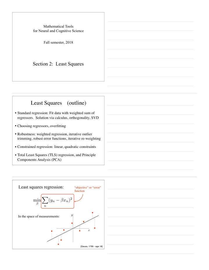Solution via calculus, orthogonality, SVD • Choosing regressors, overfitting • Robustness: weighted regression, iterative outlier trimming, robust error functions, iterative re-weighting • Constrained regression: linear, quadratic constraints • Total Least Squares (TLS) regression, and Principle Components Analysis (PCA) Least squares regression: “objective” or “error" function X ( y n − β x n ) 2 min β n In the space of measurements: y x [Gauss, 1795 - age 18]

“objective function” Error Error Error Error Error Error Error Error Error y y y y y y y y y β β β β β β β β x x x x x x x x β x Optimum X ( y n − β x n ) 2 min β n can solve this with calculus... [on board]

... or linear algebra: ( y n − β x n ) 2 = min X x || 2 min β || ~ y − �~ β n Observation Regressor Residual error ~ ~ y x 30 30 30 25 25 25 20 20 20 β = − 15 15 15 10 10 10 5 5 5 0 0 0 4 2 0 − 2 1 0.5 0 2 0 − 2 ... or linear algebra: ( y n − β x n ) 2 = min X x || 2 min β || ~ y − �~ β n Geometry: Note: this is not the 2D (x,y) measurement space of previous plots! β opt

Multiple x k || 2 = min X y − X ~ � || 2 || ~ � k ~ || ~ min y − regression: ~ ~ � � k Observation ~ ~ ~ ~ x 1 x 2 y x 0 30 30 30 30 25 25 25 25 20 20 20 20 β 0 β 1 β 2 15 − 15 − 15 − 15 10 10 10 10 5 5 5 5 0 0 0 0 1 0.5 0 1 0.5 0 0.5 0 − 0.5 0.2 0.1 0 Solution via the Orthogonality Principle Construct matrix , containing columns and ~ ~ X x 1 x 2 X T ⇣ ⌘ y − X ~ Orthogonality condition: = ~ ~ � 0 { ~ y 2D vector space Error containing all linear vector combinations of ~ x 1 and ~ ~ x 2 x 2 X ~ � opt ~ x 1 Alternatively, use SVD... Solution: β ∗ opt ,k = y ∗ k /s k , for each k ~ opt = S # ~ or � ∗ y ∗ [on board: transformations, elliptical geometry]

Optimization problems Heuristics, exhaustive search, (pain & suffering) Smooth (C 2 ) Iterative descent, Convex (possibly) nonunique Quadratic Iterative descent, guaranteed Closed-form guaranteed statAnMod - 9/12/07 - E.P. Simoncelli Interpretation: what does it mean? Note that these all give the same regression fit: [Anscombe, 1973] Polynomial regression - how many terms?

“True” model error Error Empirical (data) error Model complexity (to be continued, when we get to “statistics”...) Weighted Least Squares X [ w n ( y n − β x n )] 2 min β n x ) || 2 = min β || W ( ~ y − �~ diagonal matrix Solution via simple extensions of basic regression solution (i.e., let and and solve for ) y ∗ = W ~ x ∗ = W ~ ~ y ~ x β “outlier” 1 0.5 0 true value − 0.5 observed data regression fit − 2 − 1 0 1 2 Solution 1: “trimming”...

1 0.5 0 true value observed data − 0.5 regression fit trimmed regression − 2 − 1 0 1 2 When done iteratively (discard the outlier, re-fit, repeat), this is a so-called “greedy” method. When do you stop? Solution 2: Use a “robust” error metric. For example: f ( d ) = d 2 f ( d ) = log( c 2 + d 2 ) “Lorentzian” Note: generally can’t obtain solution directly (i.e., requires an iterative optimization procedure). In some cases, can use iteratively re-weighted least squares (IRLS)... Iteratively Re-weighted Least Squares (IRLS) d 2 f ( d ) initialize: w (0) = 1 n β ( i ) = arg min n [( y n − β x n )] 2 X w ( i ) β n iterate f ( y n − β ( i ) x n ) w ( i +1) = n ( y n − β ( i ) x n ) 2 (one of many variants)

Constrained Least Squares Linear constraint: y − X ~ c · ~ � || 2 , || ~ min where ~ � = ↵ ~ � Quadratic constraint: � || 2 = 1 y − X ~ where || C ~ � || 2 , || ~ min ~ � Both can be solved exactly using linear algebra (SVD)... [on board, with geometry] Standard Least Squares regression objective: Squared error of the “dependent” variable y x x || 2 β || ~ y − �~ min Total Least Squares Regression (a.k.a “orthogonal regression”) Error is squared distance from the fitted line... y x u || 2 = 1 u || 2 , min u || D ˆ where || ˆ ˆ Note: “data” now includes both x and y coordinates

|| USV T ˆ u || 2 = || SV T ˆ u || 2 = || S ˆ u ∗ || 2 = || ~ u ∗∗ || 2 , ~ u ∗∗ min max where D = USV T , u ∗ = V T ˆ u ∗∗ = S ˆ ˆ u, ~ u ∗ ˆ u ∗ ˆ u V T S V Set of ’s of Set of ’s of ˆ u ∗ ˆ u length 1 length 1 First two components (i.e., unit vectors) (i.e., unit vectors) of (rest are zero!), ~ u ∗∗ for three example ’s. S Eigenvectors/eigenvalues Define symmetric matrix: , the k th columns of , ~ V v k is called an eigenvector of C : V ( S T S ) V T ~ M T M C = C ~ v k = v k ( USV T ) T ( USV T ) V ( S T S )ˆ = = e k V S T U T USV T s 2 = = k V ˆ e k V ( S T S ) V T s 2 = = k ~ v k • “rotate, stretch, rotate back” • output is a rescaled copy of input • matrix C “summarizes” the • scale factor is called the s 2 k shape of the data eigenvalue associated with ~ v k Eigenvectors/eigenvalues If is the k th column of then: Define symmetric matrix: ~ V v k V ( S T S ) V T ~ M T M C = C ~ v k = v k ( USV T ) T ( USV T ) V ( S T S )ˆ = = e k V S T U T USV T s 2 = = k V ˆ e k V ( S T S ) V T s 2 = = k ~ v k And, for arbitrary vectors : ~ x X s 2 v T C ~ x = k ( ~ k ~ x ) ~ v k k