
SLIDE 1
Learning Visual Semantics: Models, Massive Computation, and - - PowerPoint PPT Presentation
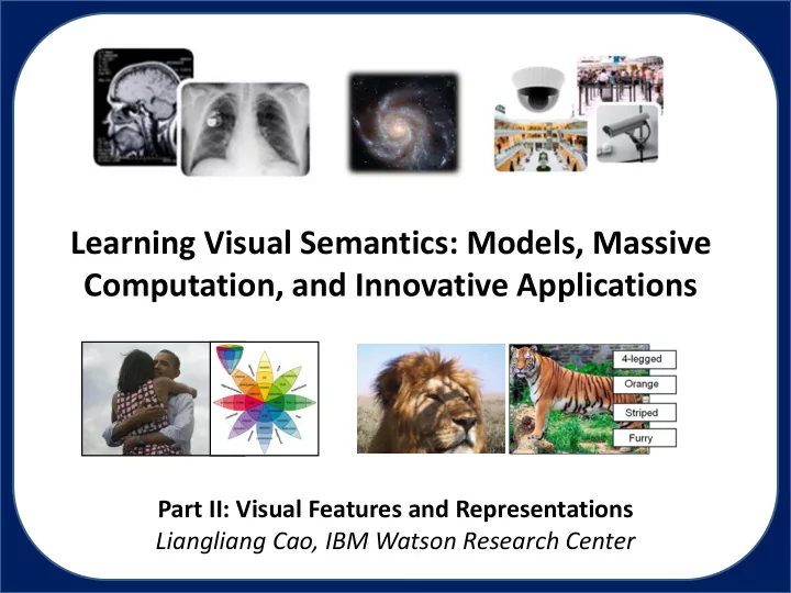
Learning Visual Semantics: Models, Massive Computation, and Innovative Applications Part II: Visual Features and Representations Liangliang Cao, IBM Watson Research Center Evolvement of Visual Features Low level features and histogram
2
3
Less parameters More parameters
4
5
Concatenating raw pixels as 1D vector
Pictures courtesy to Face Research Lab, Antonio Torralba and Sam Roweis Application 1: Face recognition Application 2: Hand written digits Tiny Image [Torralba et al 2007]: resize an image to 32x32 color thumbnail, which corresponds to a 3072 dimensional vector
7
b g r
Similar color histogram feature
8
Example thanks to Erik Learned-Miller
The same histogram!
Ojala et al, PAMI’02
[Lazebnik et al CVPR’06]
9
First position in 1st and 2nd ImageCLEF Medical Imaging Classification
10
First position in 1st and 2nd ImageCLEF Medical Imaging Classification http://www.imageclef.org/2012/medical
11
Widely used in fingerprint, iris, OCR, texture and face recognition.
12
1999 SIFT features and beyond
Classical features
13
14
15
16
dim = # codewords
17
dim = #codewords x #grids
18
19
20
Sivic et al. ICCV 2005
Fei-Fei et al. CVPR 2005 Cao and Fei-Fei. ICCV 2007
21
22
23
24
Sparse coding + spatial pyramid + linear SVM
25
[J. Wang et al CVPR10] Matlab implementation (http://www.ifp.illinois.edu/~jyang29/LLC.htm ) Can be further speed up for top-k search
26
s.t. Sparsest solution! Less sparse!
27
28
29
30
Component 1 Component 2 Component 3
31
Component 1 Component 2 Component 3
32
GMM pooling HOG LBP
33
34
35
36
A 10 line binary SVM solver by Shai Shalev-Shwartz decreasing learning rate
37
38
http://smith-gpu.pok.ibm.com:8080/
40
www.ibm.com/watsonjobs Watson is hiring!
contact zhou@us.ibm.com
41
42
Histogram Sparse coding (10K parameters) Supervec, Fishervec (0.4M parameters) Deep CNN (60M para) Bigger Small dataset
(e.g., Caltech101, 8K im)
Medium dataset
(e.g., PASCAL, 10+K)
Large dataset
(e.g., ImageNet 1.2M)
Bigger