learning algorithms for dynamic pricing a comparative
play

Learning Algorithms for Dynamic Pricing: A Comparative Study - PDF document

ICML 2020 Workshop on Real World Experiment Design and Active Learning Learning Algorithms for Dynamic Pricing: A Comparative Study Chaitanya Amballa 1 , Narendhar Gugulothu 1 , Manu K. Gupta 2 and Sanjay P. Bhat 1 1 TCS Research and Innovation


  1. ICML 2020 Workshop on Real World Experiment Design and Active Learning Learning Algorithms for Dynamic Pricing: A Comparative Study Chaitanya Amballa 1 , Narendhar Gugulothu 1 , Manu K. Gupta 2 and Sanjay P. Bhat 1 1 TCS Research and Innovation Labs, India 2 Department of Management Studies, Indian Institute of Technology, Roorkee, India Abstract We consider the problem of dynamic pricing, or time-based pricing in which businesses set flexible prices for products or services based on current market demands. Various learning algorithms have been explored in literature for dynamic pricing with the goal of achieving the minimal regret. We present a comparative experimental study of the relative performance of these learning algorithms as well as two practical improvements in the context of dynamic pricing, and list the resulting insights. Performance is measured in terms of expected cumulative regret, which is the expected regret of not suggesting the best price in hindsight. Keywords: Thompson sampling, Dynamic pricing, Exploration strategies, Regret. 1. Introduction One of the most important problem any retailer has to solve is, how to price items correctly without accurate prior knowledge of the true demand. One method to learn the demand function is price experimentation, where retailer adaptively modify prices to learn the hidden demand function and use that to estimate the revenue-maximizing price. Nevertheless, proper price experimentation is a challenging problem as the potential revenue loss during the learning horizon can be substantially large. In fact optimally balancing the trade- off between randomly selecting prices to expedite the learning versus selecting prices that maximize the expected earning has been the subject of recent research in dynamic pricing literature (see Keskin and Zeevi (2014), den Boer and Zwart (2014)). While the primary research trend in this field has been to study the performance of a given learning algorithm, this paper focuses on the comparison of various learning frameworks.
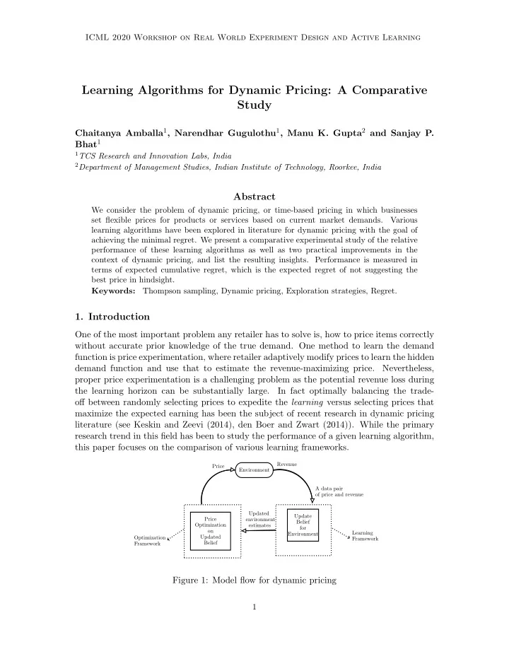
 Revenue Price Environment A data pair of price and revenue Updated Update Price environment Belief Optimization estimates for on Learning Environment Updated Optimization Framework Belief Framework Figure 1: Model flow for dynamic pricing 1

  2. Workshop on Real World Experiment Design and Active Learning Figure 1 shows a general framework for the dynamic pricing problem where environment generates revenue based on the unknown demand curve and some price as an input. The learning framework updates its belief (that is, learns the demand curve) based on the price and revenue pair (input data). The optimization framework suggests the best (optimal) price based on its current belief (estimate) of the environment. In a dynamic pricing setting, the objective is to learn the optimal price as quickly as possible. 2. Model description Suppose a firm sells a product over a time horizon of T periods. In each period t = 1 , 2 , . . . T, the seller must choose a price p t from a given feasible set [ p min , p max ] ∈ R , where 0 ≤ p min < p max < ∞ . The seller observes the demand d t according to the following linear demand model d t = α − βp t + ξ t for t = 1 , 2 , . . . , T, where α, β > 0 represent the parameters of the unknown demand model, and ξ t ∼ N (0 , σ 2 ) represents unobserved demand perturbations. The seller’s single period revenue r t in period t equals r t = d t p t . This leads to a quadratic dependence of r t on p t . More generally, one can consider demand models that lead to a higher degree polynomial dependence of revenue on the price. Hence, we consider a general µ 2 p 2 µ n p n polynomial for the revenue function r t = g ( p t )+ ξ t , where g ( p t ) = ˜ µ 0 +˜ µ 1 p t +˜ t + · · · +˜ t . The firm’s goal is to learn the unknown parameters ˜ µ 0 , ˜ µ 1 , · · · , ˜ µ n from noisy observations of price and revenue pairs { ( p t , r t ) } T t =1 well enough to reduce the T -period expected regret, defined as T [ r ∗ − E ( r t )] , � R ( T ) = t =1 where r ∗ = p ∈ [ p min ,p max ] g ( p ) is the optimal expected single period revenue. For each positive max integer n , define f n : R → R n +1 by f n ( p ) = [1 , p, p 2 , . . . , p n ] T . On denoting x t = f n ( p t ), we µ T x t with ˜ see that E ( g ( p t ) | x t ) = ˜ µ = [˜ µ 0 , ˜ µ 1 , · · · ˜ µ n ]. Thus, the dynamic pricing problem as posed above can be cast as stochastic linear optimization problem with bandit feedback. In subsequent sections, we discuss several algorithms to learn the unknown parameters of the polynomial g ( · ) for the above bandit optimization problem. 3. Different algorithms for dynamic pricing In this section, we discuss various learning algorithms for dynamic pricing. First, we present some simple baseline methods which have known theoretical guarantees in terms of regret bounds (see Keskin and Zeevi (2014)). 3.1 Baseline algorithms The two methods for dynamic pricing that we consider as baselines are: 1) Iterated least square (ILS) and 2) Constrained iterated least square (CILS). ILS estimates the revenue curve by applying least squares to the set of prior prices and realized demands, and then selects the price for the next period greedily with respect to the estimated revenue curve. ILS has been shown to be sub-optimal, while CILS has been shown to achieve asymptoti- cally optimal regret (see Keskin and Zeevi (2014)). CILS achieves asymptotically optimal regret by integrating forced price-dispersion with ILS. More precisely, CILS with threshold 2

  3. ICML 2020 Workshop on Real World Experiment Design and Active Learning parameter k suggests at time t the price � p t − 1 + sgn( δ t ) kt − 1 / 4 if | δ t | < kt − 1 / 4 , ¯ p t = ILS price otherwise. where δ t = p t − 1 − ¯ p t − 1 as the average of the prices suggested over t − 1 periods. p t − 1 , with ¯ 3.2 Action Space Exploration Action Space Exploration (ASE) (see Watkins (1989); Vemula et al. (2019)), in principle, combines ILS with the ǫ -greedy exploration strategy, which is one of the simplest and most widely used strategies for exploration. More precisely, at each decision instant, action space exploration updates the estimates of the parameters of the revenue curve by using gradient descent on the mean-square error (MSE) loss between the estimated and true revenue curve computed on the price-revenue pairs observed till then. It then selects a random price with probability ǫ , and selects the price that is greedy with respect to the updated estimate of the revenue curve with complementary probability 1 − ǫ . For the experimental results, we have used ǫ -greedy strategy with exponentially decreasing ǫ (see Vermorel and Mohri (2005)). Due to space constraints, we refrain from giving a detailed algorithm here, and instead refer the reader to the papers cited above. 3.3 Parameter Space Exploration Parameter Space Exploration (PSE) has been studied in Fortunato et al. (2017); Plappert et al. (2017); Miyamae et al. (2010); Wang et al. (2018); R¨ uckstiess et al. (2010); Neelakantan et al. (2015) and used in reinforcement learning, control and ranking tasks. Like Thompson sampling, parameter space exploration also, in essence, maintains a posterior distribution over the parameters of the revenue curve, and selects a price that is greedy with respect to a parameter vector w sampled from the posterior. The sampling is achieved by perturbing the current estimated parameter vector ˆ µ with a zero-mean, uncorrelated Gaussian noise vector σ ◦ ˆ ǫ , where ˆ ǫ is a vector of independent samples of a standard normal random variable. The ˆ parameter estimate ˆ µ and standard deviations ˆ σ of the Gaussian noise variables are updated as in Plappert et al. (2017) by using gradient descent on the mean-square error (MSE) loss between the sampled and true revenue curves on the price-revenue pairs observed till then. The detailed algorithm is presented as Algorithm 1 in Appendix A. 3.4 Thompson Sampling We use Bayesian linear regression with Thompson sampling (TS) for learning the unknown parameters. At time t , TS maintains a multivariate Gaussian posterior distribution with mean µ t and covariance A t ∈ R n × n over the unknown parameters. At time t +1, TS chooses the price p t +1 greedily according to a parameter vector w t sampled from the prior at time t . This results in a new observation r t +1 of the revenue. The new observation is used to update the posterior distribution according to the following update equations (see Bagnell (2005) for details). A − 1 t +1 = A − 1 + σ − 2 x t +1 x T t +1 , and A − 1 t +1 µ t +1 = A − 1 t µ t + σ − 2 r t +1 x t +1 , (1) t 3

Download Presentation
Download Policy: The content available on the website is offered to you 'AS IS' for your personal information and use only. It cannot be commercialized, licensed, or distributed on other websites without prior consent from the author. To download a presentation, simply click this link. If you encounter any difficulties during the download process, it's possible that the publisher has removed the file from their server.

Recommend


More recommend