lattice theoretic data flow analysis framework lattices
play

Lattice-Theoretic Data Flow Analysis Framework Lattices Define - PDF document

Lattice-Theoretic Data Flow Analysis Framework Lattices Define lattice D = ( S , ): Goals: provide a single, formal model that describes all DFAs S is a (possibly infinite) set of elements is a binary relation over elements of


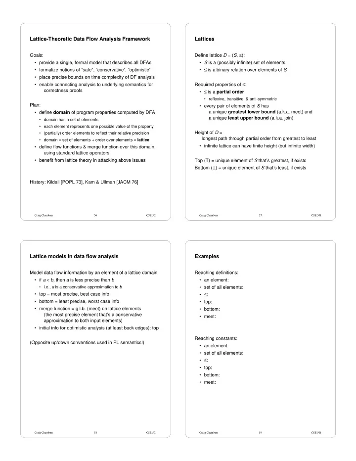
  1. Lattice-Theoretic Data Flow Analysis Framework Lattices Define lattice D = ( S , ≤ ): Goals: • provide a single, formal model that describes all DFAs • S is a (possibly infinite) set of elements • ≤ is a binary relation over elements of S • formalize notions of “safe”, “conservative”, “optimistic” • place precise bounds on time complexity of DF analysis Required properties of ≤ : • enable connecting analysis to underlying semantics for correctness proofs • ≤ is a partial order • reflexive, transitive, & anti-symmetric Plan: • every pair of elements of S has a unique greatest lower bound (a.k.a. meet) and • define domain of program properties computed by DFA a unique least upper bound (a.k.a. join) • domain has a set of elements • each element represents one possible value of the property Height of D = • (partially) order elements to reflect their relative precision longest path through partial order from greatest to least • domain = set of elements + order over elements = lattice • infinite lattice can have finite height (but infinite width) • define flow functions & merge function over this domain, using standard lattice operators • benefit from lattice theory in attacking above issues Top (T) = unique element of S that’s greatest, if exists Bottom ( ⊥ ) = unique element of S that’s least, if exists History: Kildall [POPL 73], Kam & Ullman [JACM 76] Craig Chambers 56 CSE 501 Craig Chambers 57 CSE 501 Lattice models in data flow analysis Examples Model data flow information by an element of a lattice domain Reaching definitions: • if a < b , then a is less precise than b • an element: • i.e., a is a conservative approximation to b • set of all elements: • ≤ : • top = most precise, best case info • bottom = least precise, worst case info • top: • merge function = g.l.b. (meet) on lattice elements • bottom: (the most precise element that’s a conservative • meet: approximation to both input elements) • initial info for optimistic analysis (at least back edges): top Reaching constants: (Opposite up/down conventions used in PL semantics!) • an element: • set of all elements: • ≤ : • top: • bottom: • meet: Craig Chambers 58 CSE 501 Craig Chambers 59 CSE 501

  2. Some typical lattice domains Tuples of lattices Powerset lattice: set of all subsets of a set S Often helpful to break down a complex lattice into a tuple of • ordered by ⊆ or ⊇ lattices, one per variable/stmt/... being analyzed • top & bottom = ∅ & S , or vice versa Formally: D T = <S T , ≤ T > (D = <S, ≤ >) N = • height = | S | (infinite if S is infinite) • S T = S 1 × S 2 × ... × S N • “a collecting analysis” • element of tuple domain is a tuple of elements from each variable’s domain • i th component of tuple is info about i th variable/stmt/... A lifted set: a set of incomparable values, plus top & bottom • <..., d 1 i , ...> ≤ T <..., d 2 i , ...> ≡ d 1 i ≤ d 2 i , ∀ i • e.g., reaching constants domain, for a particular variable: • i.e. pointwise ordering T • meet: pointwise meet ... x=-2 x=-1 x=0 x=1 x=2 ... • top: tuple of tops • bottom: tuple of bottoms ⊥ • height(D T ) = N * height(D) • height = 3 (even though width is infinite!) Two-point lattice: top and bottom Powerset( S ) lattice is isomorphic to a tuple of two-point lattices, • computes a boolean property one two-point lattice element per element of S • i.e., a bit-vector! Single-point lattice: just bottom • trivial do-nothing analysis Craig Chambers 60 CSE 501 Craig Chambers 61 CSE 501 Example: reaching constants Analysis of loops in lattice model How to model reaching constants for all variables? Consider: d entry d backedge d head Informally: each element is a set of the form {..., x → k , ...}, with at most one binding for x B One lattice model: a powerset of all x → k bindings • S = pow({ x → k | ∀ x , ∀ k }) • ≤ = ⊆ (Assume B (d head ) computes d backedge ) • height? Want solution to constraints: Another lattice model: d head = d entry ∩ d backedge N -tuple of 3-level constant prop. lattices, for each of N variables d backedge = B (d head ) T Let F (d) = d entry ∩ B (d) ) N • ( ... x=-2 x=-1 x=0 x=1 x=2 ... ⊥ Then want fixed-point of F : • height? d head = F (d head ) Are they the same? If not, which is better? Craig Chambers 62 CSE 501 Craig Chambers 63 CSE 501

  3. Iterative analysis in lattice model Termination of iterative analysis Iterative analysis computes fixed-point In general, k need not be finite by iterative approximation: Sufficient conditions for finiteness: F 0 = d entry ∩ T = d entry • flow functions (e.g. F ) are monotonic • lattice is of finite height F 1 = d entry ∩ B ( F 0 ) = F ( F 0 ) = F (d entry ) A function F is monotonic iff: F 2 = d entry ∩ B ( F 1 ) = F ( F 1 ) = F ( F ( F 0 )) = F ( F (d entry )) d 2 ≤ d 1 ⇒ F (d 2 ) ≤ F (d 1 ) • for application of DFA, this means that giving a flow function . . . at least as conservative inputs (d 2 ≤ d 1 ) leads to at least as conservative outputs ( F (d 2 ) ≤ F (d 1 )) F k = d entry ∩ B ( F k -1 ) = F ( F k -1 ) = F ( F (...( F (d entry ))...)) For monotonic F over domain D , the maximum number of times until that F can be applied to itself, starting w/ any element of D, w/o reaching fixed-point, is height( D )-1 F k +1 = d entry ∩ B ( F k ) = F ( F k ) F k = • start at top of D • for each application of F, either it’s a fixed-point, or the result must go down at least one level in lattice Is k finite? • eventually must hit a fixed-point If so, how big can it be? (which will be the best fixed-point) or bottom (which is guaranteed to be a fixed-point), if D of finite height Craig Chambers 64 CSE 501 Craig Chambers 65 CSE 501 Complexity of iterative analysis Another example: integer range analysis How long does iterative analysis take? For each program point, for each integer-typed variable, calculate (an approximation to) the set of integer values l : depth of loop nesting that can be taken on by the variable n : # of stmts in loop • use info for constant folding comparisons, t : time to execute one flow function for eliminating array bounds checks, k : height of lattice for (in)dependence testing of array accesses, for eliminating overflow checks What domain to use? • what is its height? What flow functions to use? • are they monotonic? Craig Chambers 66 CSE 501 Craig Chambers 67 CSE 501

  4. Example Widening operators If domain is tall, then can introduce artificial generalizations for i := 0 to N-1 (called widenings ) when merging at loop heads ... a[i] ... end • ensure that only a finite number of widenings are possible • not easy to design the “right” widening strategy i := 0 i <= N-1? ... i >= 0 && i < N? t := a[i] ... i := i + 1 Craig Chambers 68 CSE 501 Craig Chambers 69 CSE 501 A generic worklist algorithm for lattice-theoretic DFA Sharlit Maintain a mapping from each program point to info at that point A data flow analyzer generator [Tjiang & Hennessy 92] • optimistically initialize all pp’s to T • analogous to YACC Set initial pp’s (e.g. entry/exit point) to their correct values User writes basic primitives: • control flow graph representation Maintain a worklist of nodes whose flow functions need to be • nodes are instructions, not basic blocks evaluated • domain (“flow value”) representation and key operations • initialize with all nodes in graph • init • include explicit meet & widening-meet nodes • copy • is_equal While worklist nonempty do • meet • flow functions for each kind of instruction Remove a node from worklist • action routines to optimize after analysis Evaluate the node’s flow function, given current info on predecessor/successor pp’s, allowing it to change info on predecessor/successor pp’s Sharlit generates iterative dataflow analyzer from these pieces If any pp info changed, then put adjacent nodes on worklist + easy to build, extend (if not already there) − not highly efficient, so far... For faster analysis, want to follow topological order • number nodes in topological order • remove nodes from worklist in increasing topological order Craig Chambers 70 CSE 501 Craig Chambers 71 CSE 501

Download Presentation
Download Policy: The content available on the website is offered to you 'AS IS' for your personal information and use only. It cannot be commercialized, licensed, or distributed on other websites without prior consent from the author. To download a presentation, simply click this link. If you encounter any difficulties during the download process, it's possible that the publisher has removed the file from their server.

Recommend


More recommend