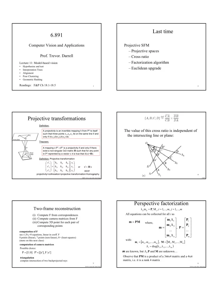
last time 6 891
play

Last time 6.891 Computer Vision and Applications Projective SFM - PDF document

Last time 6.891 Computer Vision and Applications Projective SFM Projective spaces Prof. Trevor. Darrell Cross ratio Factorization algorithm Lecture 11: Model-based vision Hypothesize and test Euclidean upgrade


  1. Last time 6.891 Computer Vision and Applications Projective SFM – Projective spaces Prof. Trevor. Darrell – Cross ratio – Factorization algorithm Lecture 11: Model-based vision • Hypothesize and test – Euclidean upgrade • Interpretation Trees • Alignment • Pose Clustering • Geometric Hashing Readings: F&P Ch 18.1-18.5 1 2 Projective transformations Definition: The value of this cross ratio is independent of A projectivity is an invertible mapping h from P 2 to itself such that three points x 1 ,x 2 ,x 3 lie on the same line if and the intersecting line or plane: only if h (x 1 ), h (x 2 ), h (x 3 ) do. Theorem: A mapping h : P 2 → P 2 is a projectivity if and only if there exist a non-singular 3x3 matrix H such that for any point in P 2 reprented by a vector x it is true that h (x)= H x Definition: Projective transformation  x '   h h h   x   1  11 12 13  1    x ' = h h h x     x' = H x or   2 21 22 23 2       x ' h h h x       8DOF 3 31 32 33 3 projectivity=collineation=projective transformation=homography 3 4 [F&P, www.cs.unc.edu/~marc/mvg] [F&P] Perspective factorization Two-frame reconstruction = P = = λ m M , i 1 ,..., m , j 1 ,..., m ij ij i j All equations can be collected for all i as (i) Compute F from correspondences (ii) Compute camera matrices from F  Λ    m P m = 1 1 1 PM (iii)Compute 3D point for each pair of where,     Λ m P corresponding points     = 2 2 = 2 m , P     ... ... computation of F     use x‘ i Fx i =0 equations, linear in coeff. F Λ m P     n n m 8 points (linear), 7 points (non-linear), 8+ (least-squares) with: (more on this next class) [ ] [ ] = = m m , m ,..., m , M M , M ,..., M i i 1 i 2 im 1 2 m computation of camera matrices ( ) Λ = diag λ , λ ,..., λ i i 1 i 2 im Possible choice: m are known, but Λ i , P and M are unknown… = = P [I | 0] P' [[e' ] F | e' ] × Observe that PM is a product of a 3 m x4 matrix and a 4x n triangulation matrix, i.e. it is a rank 4 matrix compute intersection of two backprojected rays 5 6 [www.cs.unc.edu/~marc/mvg] [www.cs.unc.edu/~marc/mvg] 1

  2. Iterative perspective factorization When Λ i are unknown the following algorithm can be used: Euclidean upgrade 1. Set λ ij =1 (affine approximation). Given a camera with known intrinsic parameters, we 2. Factorize PM and obtain an estimate of P and M . If s 5 is can take the calibration matrix to be the identity and sufficiently small then STOP. write the perspective projection equation in some 3. Use m , P and M to estimate Λ i from the camera equations Euclidean world coordinate system as (linearly) m i Λ i = P i M 4. Goto 2. In general the algorithm minimizes the proximity measure for any non-zero scale factor λ . If M i and P j denote the P ( Λ , P , M )=s 5 shape and motion parameters measured in some Euclidean coordinate system, there must exist a 4 × 4 Structure and motion recovered up to an arbitrary projective matrix Q such that transformation 7 8 [www.cs.unc.edu/~marc/mvg] [F&P] Today: “Model-based Vision” Approach Still feature and geometry-based, but now • Given with moving objects rather than cameras… – CAD Models (with features) Topics: – Detected features in an image • Hypothesize and test recognition… – Hypothesize and test – Interpretation Trees – Guess – Alignment – Render – Pose Clustering – Compare – Invariances – Geometric Hashing 9 10 Features? Hypothesize and Test Recognition • Hypothesize object identity and correspondence • Points – Recover pose – Render object in camera but also, – Compare to image • Lines • Issues – where do the hypotheses come from? • Conics – How do we compare to image (verification)? • Other fitted curves • Regions (particularly the center of a region, etc.) 11 12 2

  3. How to generate hypotheses? Interpretation Trees • Brute force • Tree of possible model-image feature assignments – Construct a correspondence for all object features to • Depth-first search every correctly sized subset of image points • Prune when unary (binary, …) constraint violated – Expensive search, which is also redundant. – length – L objects with N features – area – M features in image – orientation – O(LM N ) ! (a,1) • Add geometric constraints to prune search, leading (b,2) … to interpretation tree search … • Try subsets of features (frame groups)… 13 14 Interpretation Trees Adding constraints • Correspondences between image features and model features are not independent. • A small number of good correspondences yields a reliable pose estimation --- the others must be consistent with this. • Generate hypotheses using small numbers of correspondences (e.g. triples of points for a calibrated perspective camera, etc., etc.) “Wild cards” handle spurious image features [ A.M. Wallace. 1988. ] 15 16 Alignment Pose consistency / Alignment • Given known camera type in some unknown configuration (pose) – Hypothesize configuration from set of initial features – Backproject – Test • “Frame group” -- set of sufficient correspondences to estimate configuration, e.g., – 3 points – intersection of 2 or 3 line segments, and 1 point 17 18 3

  4. Pose clustering • Each model leads to many correct sets of correspondences, each of which has the same pose • Vote on pose, in an accumulator array (per object) 19 20 Pose Clustering 21 22 Pose clustering pick feature pair Problems – Clutter may lead to more votes than the target! – Difficult to pick the right bin size Confidence-weighted clustering – See where model frame group is reliable (visible!) – Downweight / discount votes from frame groups at poses where that frame group is dark regions show reliable views of those unreliable… 23 24 features 4

  5. 25 26 27 28 Detecting 0.1% inliers among 99.9% outliers? Lowe’s Model verification step • Example: David Lowe’s SIFT-based Recognition system • Examine all clusters with at least 3 features • Goal: recognize clusters of just 3 consistent features • Perform least-squares affine fit to model. among 3000 feature match hypotheses • Discard outliers and perform top-down check for • Approach additional features. – Vote for each potential match according to model ID and pose • Evaluate probability that match is correct – Insert into multiple bins to allow for error in similarity – Use Bayesian model, with probability that features approximation would arise by chance if object was not present – Using a hash table instead of an array avoids need to – Takes account of object size in image, textured regions, form empty bins or predict array size model feature count in database, accuracy of fit (Lowe, CVPR 01) 29 30 [Lowe] [Lowe] 5

  6. Solution for affine parameters Models for planar surfaces with SIFT keys: • Affine transform of [x,y] to [u,v]: • Rewrite to solve for transform parameters: 31 32 [Lowe] [Lowe] 3D Object Recognition Planar recognition • Extract outlines with background • Planar surfaces can be subtraction reliably recognized at a rotation of 60° away from the camera • Affine fit approximates perspective projection • Only 3 points are needed for recognition 33 34 [Lowe] [Lowe] 3D Object Recognition Recognition under occlusion • Only 3 keys are needed for recognition, so extra keys provide robustness • Affine model is no longer as accurate 35 36 [Lowe] [Lowe] 6

  7. Robot Localization Location recognition • Joint work with Stephen Se, Jim Little 37 38 [Lowe] [Lowe] Map continuously built over time Locations of map features in 3D 39 40 [Lowe] [Lowe] Invariance Invariant recognition • There are geometric properties that are invariant to camera transformations • Affine invariants • Easiest case: view a plane object in scaled – Planar invariants orthography. – Geometric hashing • Assume we have three base points P_i on the • Projective invariants object – Determinant ratio – then any other point on the object can be written as • Curve invariants ( ) + µ kb P ( ) k = P 1 + µ ka P 2 − P 3 − P P 1 1 41 42 7

Download Presentation
Download Policy: The content available on the website is offered to you 'AS IS' for your personal information and use only. It cannot be commercialized, licensed, or distributed on other websites without prior consent from the author. To download a presentation, simply click this link. If you encounter any difficulties during the download process, it's possible that the publisher has removed the file from their server.

Recommend


More recommend