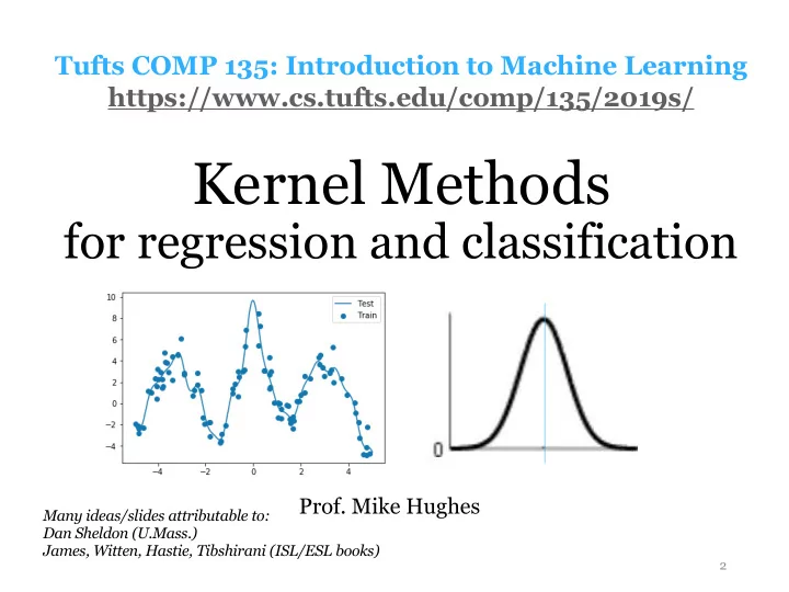
Kernel Methods for regression and classification Prof. Mike Hughes - PowerPoint PPT Presentation

Tufts COMP 135: Introduction to Machine Learning https://www.cs.tufts.edu/comp/135/2019s/ Kernel Methods for regression and classification Prof. Mike Hughes Many ideas/slides attributable to: Dan Sheldon (U.Mass.) James, Witten, Hastie, Tibshirani (ISL/ESL books) 2

Objectives for Day 19: Kernels Big idea: Use kernel functions (similarity function with special properties) to obtain flexible high-dimensional feature transformations without explicit features • From linear regression (LR) to kernelized LR • What is a kernel function? • Basic properties • Example: Polynomial kernel • Example: Squared Exponential kernel • Kernels for classification • Logistic Regression • SVMs Mike Hughes - Tufts COMP 135 - Spring 2019 3

Task: Regression & Classification y is a numeric variable Supervised e.g. sales in $$ Learning y Unsupervised Learning Reinforcement Learning x Mike Hughes - Tufts COMP 135 - Spring 2019 4

Keys to Regression Success • Feature transformation + linear model • Penalized weights to avoid overfitting Mike Hughes - Tufts COMP 135 - Spring 2019 5

Can fit linear functions to nonlinear features A nonlinear function of x: y ( x i ) = θ 0 + θ 1 x i + θ 2 x 2 i + θ 3 x 3 ˆ i φ ( x i ) = [1 x i x 2 i x 3 i ] Can be written as a linear function of 4 θ g φ g ( x i ) = θ T φ ( x i ) X y ( x i ) = ˆ g =1 “Linear regression” means linear in the parameters (weights, biases) Features can be arbitrary transforms of raw data Mike Hughes - Tufts COMP 135 - Spring 2019 6

What feature transform to use? • Anything that works for your data! • sin / cos for periodic data • polynomials for high-order dependencies φ ( x i ) = [1 x i x 2 i . . . ] • interactions between feature dimensions φ ( x i ) = [1 x i 1 x i 2 x i 3 x i 4 . . . ] • Many other choices possible Mike Hughes - Tufts COMP 135 - Spring 2019 7

Review: Linear Regression Prediction : Linear transform of G-dim features G y ( x i , θ ) = θ T φ ( x i ) = X ˆ θ g · φ ( x i ) g g =1 Training : Solve optimization problem N + L2 penalty y ( x n , θ )) 2 X min ( y n − ˆ (optional) θ n =1 Mike Hughes - Tufts COMP 135 - Spring 2019 8

Problems with high-dim features • Feature transformation + linear model How expensive is this transformation? (Runtime and storage) Mike Hughes - Tufts COMP 135 - Spring 2019 9

Thought Experiment • Suppose that the optimal weight vector can be exactly constructed via a linear combination of the training set feature vectors θ ∗ = α 1 φ ( x 1 ) + α 2 φ ( x 2 ) + . . . + α N φ ( x N ) Each alpha is a scalar Each feature vector is a vector of size G Mike Hughes - Tufts COMP 135 - Spring 2019 10

Justification? Is optimal theta a linear combo of feature vectors? Stochastic gradient descent, with 1 example per batch, can be seen as creating optimal weight vector of this form • Starting with all zero vector • In each step, adding a weight * feature vector Each update step: θ t ← θ t − 1 − η · d d θ loss( y n , θ T φ ( x n )) Let’s simplify this via chain rule! Mike Hughes - Tufts COMP 135 - Spring 2019 11

Justification? Stochastic gradient descent, with 1 example per batch, can be seen as creating optimal weight vector of this form • Starting with all zero vector • In each step, adding a weight * feature vector Each update step: θ t ← θ t − 1 − η · d da loss( y n , a ) · d d θθ T φ ( x n ) scalar scalar Vector of size G Mike Hughes - Tufts COMP 135 - Spring 2019 12

Justification? Stochastic gradient descent, with 1 example per batch, can be seen as creating optimal weight vector of this form • Starting with all zero vector • In each step, adding a weight * feature vector Each update step: θ t ← θ t − 1 − η · d da loss( y n , a ) · φ ( x n ) scalar scalar Vector of size G (simplified) Mike Hughes - Tufts COMP 135 - Spring 2019 13

How to Predict in this thought experiment θ ∗ = α 1 φ ( x 1 ) + α 2 φ ( x 2 ) + . . . + α N φ ( x N ) Prediction : y ( x i , θ ) = θ T φ ( x i ) = ˆ ! T N X y ( x i , θ ∗ ) = ˆ α n φ ( x n ) φ ( x i ) n =1 Mike Hughes - Tufts COMP 135 - Spring 2019 14

How to Predict in this thought experiment θ ∗ = α 1 φ ( x 1 ) + α 2 φ ( x 2 ) + . . . + α N φ ( x N ) Prediction : y ( x i , θ ) = θ T φ ( x i ) = ˆ N α n φ ( x n ) T φ ( x i ) X y ( x i , θ ∗ ) = ˆ n =1 Inner product of test feature vector with each training feature! Mike Hughes - Tufts COMP 135 - Spring 2019 15

Kernel Function k ( x i , x j ) = φ ( x i ) T φ ( x j ) Input: any two vectors x i and x j Output: scalar real Interpretation: similarity function for x i and x j Properties: Larger output values mean i and j are more similar Symmetric Mike Hughes - Tufts COMP 135 - Spring 2019 16

Kernelized Linear Regression • Prediction : N X y ( x i , α , { x n } N ˆ n =1 ) = α n k ( x n , x i ) = X n =1 • Training N X y ( x n , α , X )) 2 min ( y n − ˆ α n =1 Can do all needed operations with only access to kernel (no feature vectors) Mike Hughes - Tufts COMP 135 - Spring 2019 17

Compare: Linear Regression Prediction : Linear transform of G-dim features G y ( x i , θ ) = θ T φ ( x i ) = X ˆ θ g · φ ( x i ) g g =1 Training : Solve optimization problem N + L2 penalty y ( x n , θ )) 2 X min ( y n − ˆ (optional) θ n =1 Mike Hughes - Tufts COMP 135 - Spring 2019 18

Why is kernel trick good idea? Before: Training problem optimized vector of size G Prediction cost: scales linearly with G (num. high-dim features) After: Training problem optimized vector of size N Prediction cost: scales linearly with N (num. train examples) requires N evaluations of kernel So we get some saving in runtime/storage if G is bigger than N AND we can compute k faster than inner product Mike Hughes - Tufts COMP 135 - Spring 2019 19

Example: From Features to Kernels x = [ x 1 x 2 ] z = [ z 1 z 2 ] √ √ √ φ ( x ) = [1 x 2 1 x 2 2 x 1 2 x 2 2 x 1 x 2 ] 2 k ( x, z ) = (1 + x 1 z 1 + x 2 z 2 ) 2 Compare: What is relationship between these two functions defined above? φ ( x ) T φ ( z ) k ( x, z ) Mike Hughes - Tufts COMP 135 - Spring 2019 20

Example: From Features to Kernels x = [ x 1 x 2 ] z = [ z 1 z 2 ] √ √ √ φ ( x ) = [1 x 2 1 x 2 2 x 1 2 x 2 2 x 1 x 2 ] 2 k ( x, z ) = (1 + x 1 z 1 + x 2 z 2 ) 2 Compare: What is relationship between these two functions defined above? = φ ( x ) T φ ( z ) k ( x, z ) Punchline: Can sometimes find faster ways to compute high-dim. inner product Mike Hughes - Tufts COMP 135 - Spring 2019 21

Cost comparison x = [ x 1 x 2 ] z = [ z 1 z 2 ] √ √ √ φ ( x ) = [1 x 2 1 x 2 2 x 1 2 x 2 2 x 1 x 2 ] 2 k ( x, z ) = (1 + x 1 z 1 + x 2 z 2 ) 2 Compare: φ ( x ) T φ ( z ) Number of add and multiply ops to compute Number of add and multiply ops to compute k ( x, z ) Mike Hughes - Tufts COMP 135 - Spring 2019 22

Example: Kernel cheaper than inner product x = [ x 1 x 2 ] √ √ √ φ ( x ) = [1 x 2 1 x 2 2 x 1 2 x 2 2 x 1 x 2 ] 2 k ( x, z ) = (1 + x 1 z 1 + x 2 z 2 ) 2 z = [ z 1 z 2 ] φ ( x ) T φ ( z ) Compare: Number of add and multiply ops to compute 6 multiply and 5 add k ( x, z ) Number of add and multiply ops to compute 3 multiply (include square) and 2 add Mike Hughes - Tufts COMP 135 - Spring 2019 23

Squared Exponential Kernel Assume x is a scalar k ( x, z ) = e − ( x − z ) 2 max at x = z z x Also called “radial basis function (RBF)” kernel Mike Hughes - Tufts COMP 135 - Spring 2019 24

Squared Exponential Kernel Assume x is a scalar k ( x, z ) = e − ( x − z ) 2 = e − x 2 − z 2 +2 xz = e − x 2 e − z 2 e 2 xz Mike Hughes - Tufts COMP 135 - Spring 2019 25

Recall: Taylor series for e^x ∞ k ! x k = 1 + x + 1 1 e x = 2 x 2 + . . . X k =0 ∞ 2 k e 2 xz = X k ! x k z k k =0 Mike Hughes - Tufts COMP 135 - Spring 2019 26

Squared Exponential Kernel k ( x, z ) = e − ( x − z ) 2 = e − x 2 − z 2 +2 xz ∞ ! ∞ ! r r 2 k 2 k z ) = e − x 2 e − z 2 X X k ! x k k ! z k k =0 k =0 = φ ( x ) T φ ( z ) Corresponds to an INFINITE DIMENSIONAL feature vector r r r 2 k 2 0 2 1 0! x 0 e − x 2 1! x 1 e − x 2 k ! x k e − x 2 φ ( x ) = [ ] . . . . . . Mike Hughes - Tufts COMP 135 - Spring 2019 27

Kernelized Regression Demo Mike Hughes - Tufts COMP 135 - Spring 2019 28

Linear Regression Mike Hughes - Tufts COMP 135 - Spring 2019 29

Kernel Matrix for training set • K : N x N symmetric matrix   k ( x 1 , x 1 ) k ( x 1 , x 2 ) . . . k ( x 1 , x N ) k ( x 2 , x 1 ) k ( x 2 , x 2 ) . . . k ( x 2 , x N )   K = .   .   .   k ( x N , x 1 ) k ( x N , x 2 ) . . . k ( x N , x N ) Mike Hughes - Tufts COMP 135 - Spring 2019 30

Linear Regression with Kernel 100 training examples in x_train 505 test examples in x_test Mike Hughes - Tufts COMP 135 - Spring 2019 31

Linear Regression with Kernel Mike Hughes - Tufts COMP 135 - Spring 2019 32

Polynomial Kernel, deg. 5 Mike Hughes - Tufts COMP 135 - Spring 2019 33

Polynomial Kernel, deg. 12 Mike Hughes - Tufts COMP 135 - Spring 2019 34

Gaussian kernel (aka sq. exp.) Mike Hughes - Tufts COMP 135 - Spring 2019 35

Kernel Regression in sklearn Demo will use kernel=‘precomputed’ Mike Hughes - Tufts COMP 135 - Spring 2019 36