Jig 2 Split Hopkinson bar test [1] 2.1 Theory A time history of - - PDF document

18TH INTERNATIONAL CONFERENCE ON COMPOSITE MATERIALS

1 Introduction Carbon fiber reinforced plastics (CFRP) are widely used as components of structures, vehicles and so

• forth. Therefore the development of technique to

characterize material properties of CFRP for impact force is required. The split Hopkinson bar (SHPB) test is a useful technique to characterize material properties for impact loading for steels, however the effectiveness for CFRP has not been evaluated

• sufficiently. This paper evaluates the effectiveness
• f the Hopkinson bar test for CFRP by a dynamic

finite element method. 2 Split Hopkinson bar test [1] 2.1 Theory A time history of strain of a specimen is given by eq. (1),

2 ( ) { ( ) ( ) ( )}

i r t

C t t t t dt L ε ε ε ε ′ ′ ′ ′ = − − −

• (1)

where t is time, L is the length of a specimen,

) (t

r

ε

is the strain of a reflection wave,

C is the

wave velocity calculated from the Young’s modulus E and the mass density as the follows,

ρ E C =

(2) Also, the stress is given by

) ( ) ( t A A E t

t s s

ε σ =

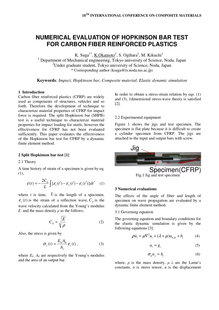
, (3) where E0 , A0 are respectively the Young’s modulus and the area of an output bar. In order to obtain a stress-strain relation by eqs. (1) and (3), 1dimensional stress-wave theory is satisfied [2]. 2.2 Experimental equipment Figure 1 shows the jigs and test specimen. The specimen is flat plate because it is difficult to create a cylinder specimen from CFRP. The jigs are attached to the input and output bars with screw. Fig.1 Jig and test specimen 3 Numerical evaluations The effects of the angle of fiber and length of specimen on wave propagation are evaluated by a dynamic finite element method. 3.1 Governing equation The governing equation and boundary conditions for the elastic dynamic simulation is given by the following equations [3]:

2 ,

( )

i i k ki i

u u u b ρ µ λ µ = ∇ + + +

• (4)

i i

u g =

(5)

ij j i

n h σ =

(6) where, is the mass density, are the Lame’s constants, is stress tensor, u is the displacement

Jig

NUMERICAL EVALUATION OF HOPKINSON BAR TEST FOR CARBON FIBER REINFORCED PLASTICS

• K. Suga1*, K.Okamoto2, S. Ogihara1, M. Kikuchi1

1 Department of Mechanical engineering, Tokyo university of Science, Noda, Japan 2Under graduate student, Tokyo university of Science, Noda, Japan

* Corresponding author (ksuga@rs.noda.tus.ac.jp)

Keywords: Impact, Hopkinson bar, Composite material, Elastic dynamic simulation

Specimen(CFRP)

vector, n is normal unit vector, g and h are the given displacement and force vectors, respectively. 3.2 Model Figure 2 shows the geometry of a numerical model

• f SHPB.

Fig.2 Numerical model of SHPB The strain of a transparent wave is observed at the position A shown in Fig. 2. A specimen of CFRP is modeled as an orthotropic material, the angle between fiber and the z-axis is defined by as shown in Fig. 3. Fig.3 Fiber angle The material constants of specimen are listed in Table 1. The input and output bars are assumed to be steel. Table 1 Material constants of specimen E1 = 9.5 Young's modulus [GPa] E2 = 9.5 E3 = 130.3 G32 = 4.7 Shear modulus [GPa] G13 = 4.7 G21 = 3.1

32

ν

= 0.34 Poisson's ratio

21

ν

= 0.5

13

ν

= 0.027 Mass density [kg/m3]

ρ

= 1800 Table 2 Material constants of input and output bar The simulations are conducted using an efficient dynamic finite element method [4]. 3.3 Conditions In order to evaluate the effect of experimental condition on estimated dynamic material properties using SHPB, the length of specimen L = 50, 150 mm , the angle = 30, 45, 60˚ and the duration time

• f impact loading T = 20, 100 s shown in Fig. 4.
• Fig. 4 Impact loading

4 Result We carried out numerical simulations under several

• conditions. We compared numerical results between

SHPB and specimen only simulation. Specimen only simulation are assumed to be ideal condition to characterize material properties, in these simulations a impact loading was applied to a specimen directly. 4.1 Length of specimen Young's modulus [GPa] E = 205 Poisson's ratio

ν

= 0.5 Mass density [kg/m3]

ρ

= 7800

x y, 2 z 1 3

• 65

Strain Gauge

z y

• x

3 NUMERICAL EVALUATION OF HOPKINSON BAR TEST FOR CARBON FIBER REINFORCED PLASTICS

Figure 5 shows the stress-strain curve for difference length of specimen, other conditions were fixed to = 0˚ and T = 20 s. In the case L = 50 mm, the trend of the stress-strain curves obtained by SHPB and specimen are in good agreement, however in the case L = 150 mm the curves are not in agreement. Fig.5 Strain-stress curve for different specimen length Figure 5.5 compares the time history of strain

• btained using specimens having the length L = 35

mm and 50 mm, the angle = 45˚. The length of specimen becomes shorter, the difference between strain histories obtained SHPB and a specimen becomes larger. The reason why the trend was

• bserved is the constraint effect by a jig is stronger

when the length of a specimen is shorter. Fig.5.5 Time history of strain for different specimen length The results Fig. 5 and 5.5 indicate an optimized length of specimen is exist to characterize material properties reasonably. 4.2 Duration time Figure 6 shows the stress-strain curves for different duration times, = 90˚ and L = 50 mm. In T = 20 s, the trend of the stress-strain curve obtained SHPB is not in agree, however in the case T = 100 s these trends are in good agreement. Fig.6 Strain-stress curve for different duration time Also, considering the stress-strain curves shown in

• Fig. 5 and 6, if the difference between the (apparent)

Young’s modulus for the z-direction and the output bar is larger, the longer duration time is required to estimate reasonable material properties using SHPB. 4.3 Angle of fiber Figure 7 shows the stress-strain curves for different angle = 30, 45, 60˚, where L = 50 mm, and T = 100

• s. The stress-strain curves estimated by SHPB are

in good agreement with the curves simulated using each specimen alone.

Fig.7 Strain-stress curve for different angle of fiber 4.4 Observation point We observed transparent waves at four different locations, A, B, C and D shown in Fig. 8. A and B are at location 50 mm away from the left of the

• utput bar, and C and D are located at 300 mm away

from it. Also A and D are located at the top, B and C are located at the side of the output bar. Fig.8 Observation points on output bar The time histories of the transparent waves are shown in Fig. 9, where = 45˚ and L = 50 mm. At A and B, the histories have significant difference because of the material anisotropy, however at C and D, the histories have same trend. These results indicate the possibility to evaluate anisotropic material properties using SHPB from the transparent waves. Fig.9 Time histories of the transparent waves for different measuring point

5 Conclusions

This study evaluated the effectiveness of the SHPB test for CFRP by numerical simulations. CFRP is modeled as an orthotropic material. The effects of the length of specimen, the duration time of impact loading and the angle of fiber on estimated material behavior by SHPB were evaluated. The simulations indicate the following remarks.

• ut SHPB test for CFRP.
• Sufficient duration time is required to obtain

reasonable stress-strain curve.

anisotropic material properties by SHPB. References

[1] U. S. Lindholm, “SOME EXPERIMENTS WITH

THE SPLIT HOPKINSON PRESSURE BAR”, J.

• Mech. Phys. Solids, Vol. 12, pp. 317-335, 1964.

[2] Bazle A Gama et al., “Hopkinson bar experimental

technique: A critical review”, Appl. Mech. Rev. 57, 4, pp. 223-249, 2004.

[3] Hughes TJR. “The Finite Element Method: Linear

Static and Dynamic Finite Element Analysis.” Dover Publications: New York, pp.490-513, 2000.

[4] K. Suga, “Efficient Dynamic Simulation Based on

Cross Section of Elastic Object”, ICM11, Lake Como, Italy, June 5-9, 2011.