Iterative improvement algorithms In many optimization problems, path - - PowerPoint PPT Presentation

Beyond Classical Search

Chapter 4, Sections 4.1-4.2

Chapter 4, Sections 4.1-4.2 1

Outline

♦ Hill-climbing ♦ Simulated annealing ♦ Genetic algorithms (briefly) ♦ Local search in continuous spaces (briefly)

Chapter 4, Sections 4.1-4.2 2

Iterative improvement algorithms

In many optimization problems, path is irrelevant; the goal state itself is the solution Then state space = set of “complete” configurations; find optimal configuration, e.g., TSP

• r, find configuration satisfying constraints, e.g., timetable

In such cases, can use iterative improvement algorithms; keep a single “current” state, try to improve it Constant space, suitable for online as well as offline search

Chapter 4, Sections 4.1-4.2 3

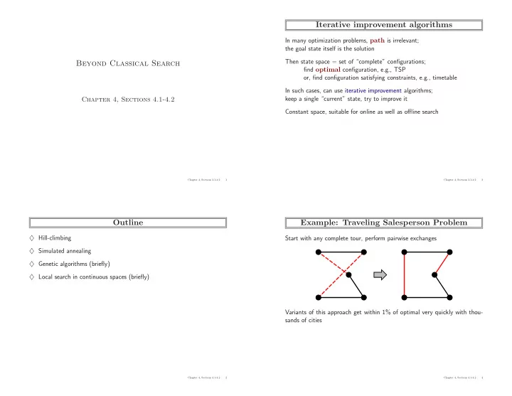
Example: Traveling Salesperson Problem

Start with any complete tour, perform pairwise exchanges Variants of this approach get within 1% of optimal very quickly with thou- sands of cities

Chapter 4, Sections 4.1-4.2 4

Example: n-queens

Put n queens on an n × n board with no two queens on the same row, column, or diagonal Move a queen to reduce number of conflicts

h = 5 h = 2 h = 0

Almost always solves n-queens problems almost instantaneously for very large n, e.g., n = 1million

Chapter 4, Sections 4.1-4.2 5

Hill-climbing (or gradient ascent/descent)

“Like climbing Everest in thick fog with amnesia”

function Hill-Climbing( problem) returns a state that is a local maximum inputs: problem, a problem local variables: current, a node neighbor, a node current ← Make-Node(Initial-State[problem]) loop do neighbor ← a highest-valued successor of current if Value[neighbor] ≤ Value[current] then return State[current] current ← neighbor end

Chapter 4, Sections 4.1-4.2 6

Hill-climbing contd.

Useful to consider state space landscape

current state

• bjective function

state space

global maximum local maximum "flat" local maximum shoulder

Random-restart hill climbing overcomes local maxima (eventually a good initial state) Random sideways moves escape from shoulders loop on flat maxima

Chapter 4, Sections 4.1-4.2 7

Ridges

Chapter 4, Sections 4.1-4.2 8

Simulated annealing

Idea: escape local maxima by allowing some “bad” moves but gradually decrease their size and frequency

function Simulated-Annealing( problem, schedule) returns a solution state inputs: problem, a problem schedule, a mapping from time to “temperature” local variables: current, a node next, a node T, a “temperature” controlling prob. of downward steps current ← Make-Node(Initial-State[problem]) for t ← 1 to ∞ do T ← schedule[t] if T = 0 then return current next ← a randomly selected successor of current ∆E ← Value[next] – Value[current] if ∆E > 0 then current ← next else current ← next only with probability e∆ E/T

Chapter 4, Sections 4.1-4.2 9

Properties of simulated annealing

At fixed “temperature” T, state occupation probability reaches Boltzman distribution p(x) = αe

E(x) kT

T decreased slowly enough = ⇒ always reach best state x∗ because e

E(x∗) kT /e E(x) kT = e E(x∗)−E(x) kT

≫ 1 for small T Is this necessarily an interesting guarantee?? Devised by Metropolis et al., 1953, for physical process modelling Widely used in VLSI layout, airline scheduling, etc.

Chapter 4, Sections 4.1-4.2 10

Local beam search

Idea: k random initial states; choose and keep top k of all their successors ♦ Not the same as k hill climbing searches run in parallel! ♦ Searches that find good states recruit other searches to join them ♦ However, if the successors from an initial state are not selected, the search starting from that state is effectively abandoned. Problem: quite often, all k states end up on same local hill Idea: ?

Chapter 4, Sections 4.1-4.2 11

Local Beam Search

Idea: k random initial states; choose and keep top k of all their successors ♦ Not the same as k hill climbing searches run in parallel! ♦ Searches that find good states recruit other searches to join them ♦ However, if the successors from an initial state are not selected, the search starting from that state is effectively abandoned. Problem: quite often, all k states end up on same local hill Idea: choose k successors randomly, biased towards good ones (Stochastic Beam Search) Observe the close analogy to natural selection!

Chapter 4, Sections 4.1-4.2 12

Genetic algorithms

= stochastic beam search + generate successors from pairs of states

32252124

Selection Cross−Over Mutation

24748552 32752411 24415124

24 23 20

32543213

11

29% 31% 26% 14%

32752411 24748552 32752411 24415124 32748552 24752411 32752124 24415411 24752411 32748152 24415417

Fitness Pairs

Chapter 4, Sections 4.1-4.2 13

Genetic algorithms contd.

GAs require states encoded as strings (GPs use programs) Crossover helps iff substrings are meaningful components

+ =

GAs = evolution: e.g., real genes encode replication machinery!

Chapter 4, Sections 4.1-4.2 14

Continuous state spaces

♦ Suppose we want to site three airports in Romania: – 6-D state space defined by (x1, y2), (x2, y2), (x3, y3) – objective function f(x1, y2, x2, y2, x3, y3) = sum of squared distances from each city to nearest airport

Chapter 4, Sections 4.1-4.2 15

Continuous state spaces–Discretization

♦ Suppose we want to site three airports in Romania: – 6-D state space defined by (x1, y2), (x2, y2), (x3, y3) – objective function f(x1, y2, x2, y2, x3, y3) = sum of squared distances from each city to nearest airport ♦ Discretization methods turn continuous space into discrete space ♦ each state has six discrete variables (e.g. ±δ miles, where δ is a constant) [or grid cells] ♦ each state has how many possible successors?

Chapter 4, Sections 4.1-4.2 16

Continuous state spaces–Discretization

♦ Suppose we want to site three airports in Romania: – 6-D state space defined by (x1, y2), (x2, y2), (x3, y3) – objective function f(x1, y2, x2, y2, x3, y3) = sum of squared distances from each city to nearest airport ♦ Discretization methods turn continuous space into discrete space ♦ each state has six discrete variables (e.g. ±δ miles, where δ is a constant) [or grid cells] ♦ each state has how many possible successors?

• 12 [book] (action: change only one variable—x or (“xor”) y of one airport)
• 36 − 1 (action: change at least one variable)

♦ what is the algorithm?

Chapter 4, Sections 4.1-4.2 17

Continuous state spaces–No Discretization

♦ Gradient (of the objective function) methods compute ∇f =

    ∂f

∂x1 , ∂f ∂y1 , ∂f ∂x2 , ∂f ∂y2 , ∂f ∂x3 , ∂f ∂y3

   

♦ To increase/reduce f, e.g., by x ← x + α∇f(x) ♦ Sometimes can solve for ∇f(x) = 0 exactly (e.g., only one airport). ♦ Otherwise, Newton–Raphson (1664, 1690) iterates x ← x−H−1

f (x)∇f(x)

to solve ∇f(x) = 0, where Hij = ∂2f/∂xi∂xj

Chapter 4, Sections 4.1-4.2 18

Contrast and Summary

♦ Ch. 3 ♦ Ch. 4.1-2 ♦ What is the key difference?

Chapter 4, Sections 4.1-4.2 19

Contrast and Summary

♦ Ch. 3: “It is the journey, not the destination.” (optimize the path) ♦ Ch. 4.1-2: “It is the destination, not the journey” (optimize the goal) ♦ Different problem formulation, do we still need:

• Initial state (state space): ?
• Successor function (actions): ?
• Step (path) cost: ?
• Goal test: ?

Chapter 4, Sections 4.1-4.2 20

Contrast and Summary

♦ Ch. 3: “It is the journey, not the destination.” (optimize the path) ♦ Ch. 4.1-2: “It is the destination, not the journey” (optimize the goal) ♦ Different problem formulation, do we still need:

• Initial state (state space): yes [but different kind of states]
• Successor function (actions): yes [but different kind of actions]
• Step (path) cost: no [not the journey]
• Goal test: no [optimize objective function]

♦ The n-queen and TSP problems can be forumluated in either way, how?

Chapter 4, Sections 4.1-4.2 21

Skipping the rest

Chapter 4, Sections 4.1-4.2 22

Searching with Non-deterministic Actions

♦ performing an action might not yield the expected successor state ♦ Suck can clean one dirty square, but sometimes an adjacent dirty square as well ♦ Suck on a clean square can sometimes make it dirty

Chapter 4, Sections 4.1-4.2 23

Erratic Vacuum World

1 2 8 7 5 6 3 4

♦ not just a sequence of actions, but backup/contingency plans ♦ from State 1: [Suck, if State = 5 then [Right, Suck] else [] ]

Chapter 4, Sections 4.1-4.2 24

And-Or Search Tree

Left Suck Right Suck Right Suck

6

GOAL

8

GOAL

7 1 2 5 1

LOOP

5

LOOP

5

LOOP Left Suck

1

LOOP GOAL

8 4

♦ every path reaches a goal, a repeated state, or a dead end

Chapter 4, Sections 4.1-4.2 25

Slippery floor

Suck Right

6 1 2 5

Right

♦

Chapter 4, Sections 4.1-4.2 26

Sensorless problems

♦ No sensor—the agent does not know which state it is in ♦ Is it hopeless?

Chapter 4, Sections 4.1-4.2 27

Belief States

♦ Each “belief” state is a collection of possible “physical” states.

L R L R S L R S S S S R L S S L R R L R L

♦ 12 “reachable” belief states (out of 255 possible belief states) ♦ If the actions have uncertain outcomes, how many belief states are there?

Chapter 4, Sections 4.1-4.2 28

Contingency problems

♦ Environment is partially observable ♦ Fixed sequence: [Suck, Right, Suck] ♦ Actions have uncertain outcomes ♦ Addtional percepts during execution: [Suck, Right, if [R Dirty] then Suck] ♦ More in Chapter 12 (Planning) ♦ Adversarial environment (e.g., games): Chapter 6

Chapter 4, Sections 4.1-4.2 29