It V T V = L In mm LV = I with L = V T LEFT INVERSE COMPSCI 527 - - PowerPoint PPT Presentation

Orthogonal Matrices

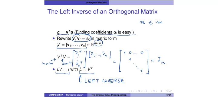
The Left Inverse of an Orthogonal Matrix

qi = vT

i p (Finding coefficients qi is easy!)

• Rewrite vT

i vj = δij in matrix form

V = [v1, . . . , vn] 2 Rm×n V TV =

• LV = I with L = V T

COMPSCI 527 — Computer Vision The Singular Value Decomposition 5 / 21

M E m

O_O

mm

It

L

In

LEFT INVERSE

Orthogonal Matrices

Left and Right Inverse of an Orthogonal Matrix

• LV = I with L = V T
• Can we have R such that VR = I?
• That would be the right inverse
• What if m = n?

COMPSCI 527 — Computer Vision The Singular Value Decomposition 6 / 21

nem

II

t.nl

mxm

rank R E n rank L E

n

I

m m

vis

m m

LV

If

all square VR Imo

El left inv

left

A anyinvertiblematrix

sight inv

LAR

R

R L

LA

I

LALR

L

If

invertible

AR

I

L

R

Orthogonal Matrices

Orthogonal Transformations Preserve Norm (m n)

y = Vx : Rn ! Rm kyk2 =

COMPSCI 527 — Computer Vision The Singular Value Decomposition 7 / 21

t d

s

m

jTy

ETV'VE

E

HEIR

HEH

1154

IIII.ATYuere

rotation

Orthogonal Projection

Projection Onto a Subspace (m  n)

• Projection of b 2 Rm onto subspace S ✓ Rm

is the point p 2 S closest to b

• Let V 2 Rm×n an orthonormal basis for S

(That is, V is an orthogonal matrix)

• b p ? vi for i = 1, . . . , n

that is, V T(b p) = 0

• Projection of b 2 Rm onto S is p = VV Tb

(optional proofs in an Appendix)

COMPSCI 527 — Computer Vision The Singular Value Decomposition 8 / 21

If

m

t

i

Es

F

VE

E WT

The Singular Value Decomposition

Linear Mappings

b = Ax : Rn → Rm. Example: A = 1 √ 2   √ 3 √ 3 −3 3 1 1   (m = n = 3) range(A) ↔ rowspace(A)

COMPSCI 527 — Computer Vision The Singular Value Decomposition 9 / 21

µ

rowspeaCA

men

E for

EIR will A

f d'm

f

EffortzelR

HYPER

ELLIPSOID

b3

I

5

x

TIFIELSPHERE

raranklA

in

e 2

Fx

Rfp cE

b

be

The Singular Value Decomposition

The Singular Value Decomposition: Geometry

b = Ax where A = 1 √ 2   √ 3 √ 3 −3 3 1 1  

COMPSCI 527 — Computer Vision The Singular Value Decomposition 10 / 21

Ari

TE

11511 1

11411 1

Tz

420

pm VI

Ariz

quiz

ate

FIL

t z Tz

th

Iwaki

Hui11 1

03 0

ctfu

O

ITE3

F

NONTRIVIAL

ITfz

REIKO

Fzspans null A

HFzH 1

Hies

L

a 3spans left hull A

T.tv 5

cities

The Singular Value Decomposition

The Singular Value Decomposition: Algebra

Av1 = σ1u1 Av2 = σ2u2 σ1 ≥ σ2 > σ3 = 0 uT

1 u1

= 1 uT

2 u2

= 1 uT

3 u3

= 1 uT

1 u2

= uT

1 u3

= uT

2 u3

= vT

1 v1

= 1 vT

2 v2

= 1 vT

3 v3

= 1 vT

1 v2

= vT

1 v3

= vT

2 v3

=

COMPSCI 527 — Computer Vision The Singular Value Decomposition 11 / 21

SMALLSVD

3

Atria

hi.info

z

Ati.int

FARGE SVD

u

I

1 I

iE

E UTAV

The Singular Value Decomposition

The Singular Value Decomposition: General

For any real m ⇥ n matrix A there exist orthogonal matrices U = ⇥ u1 · · · um ⇤ 2 Rm×m V = ⇥ v1 · · · vn ⇤ 2 Rn×n such that UTAV = Σ = diag(σ1, . . . , σp) 2 Rm×n where p = min(m, n) and σ1 . . . σp 0. Equivalently, A = UΣV T .

COMPSCI 527 — Computer Vision The Singular Value Decomposition 12 / 21

SAFEsafe

The Singular Value Decomposition

Rank and the Four Subspaces

A = UΣV T = [u1, . . . , ur, ur+1, . . . , um]            σ1 ... σr ...                       v1 . . . vr vr+1 . . . vn           

COMPSCI 527 — Computer Vision The Singular Value Decomposition 13 / 21

yr

rankcan

I

stows

pep

p 4

sperm

span spar

range lefty