Introduction to SM th. uncertainties in S Emi KOU (LPT, Universit - PowerPoint PPT Presentation

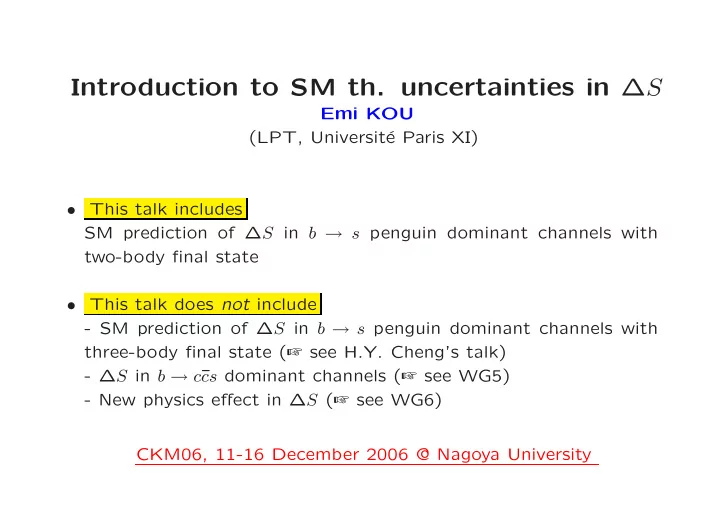
Introduction to SM th. uncertainties in ∆ S Emi KOU (LPT, Universit´ e Paris XI) • This talk includes SM prediction of ∆ S in b → s penguin dominant channels with two-body final state • This talk does not include - SM prediction of ∆ S in b → s penguin dominant channels with three-body final state ( ☞ see H.Y. Cheng’s talk) cs dominant channels ( ☞ see WG5) - ∆ S in b → c ¯ - New physics effect in ∆ S ( ☞ see WG6) CKM06, 11-16 December 2006 @ Nagoya University

Experimental status of S b → s sin(2 β eff ) ≡ sin(2 φ e ff ) H F AG H F A G 1 DPF/JPS 2006 DPF/JPS 2006 Current status of S b → s PRELIMINARY HFAG World Average 0.68 ± 0.03 b → ccs DPF/JPS 2006 BaBar 0.12 ± 0.31 ± 0.10 HFAG ➤ b → s ¯ ss dominant mode φ K 0 Belle 0.50 ± 0.21 ± 0.06 Average 0.39 ± 0.18 DPF/JPS 2006 BaBar - B → φK S : 0 . 39 ± 0 . 18 0.58 ± 0.10 ± 0.03 HFAG η′ K 0 Belle 0.64 ± 0.10 ± 0.04 Average 0.61 ± 0.07 - B → η ′ K S : 0 . 61 ± 0 . 07 DPF/JPS 2006 BaBar K S K S K S 0.66 ± 0.26 ± 0.08 HFAG Belle 0.30 ± 0.32 ± 0.08 ➤ b → s ¯ Average 0.51 ± 0.21 uu dominant mode DPF/JPS 2006 BaBar 0.33 ± 0.26 ± 0.04 HFAG π 0 K S Belle 0.33 ± 0.35 ± 0.08 - B → πK S : 0 . 33 ± 0 . 21 DPF/JPS 2006 Average 0.33 ± 0.21 HFAG BaBar 0.20 ± 0.52 ± 0.24 ρ 0 K S Average - B → ρK S : 0 . 20 ± 0 . 57 0.20 ± 0.57 DPF/JPS 2006 0.62 + 0 . 2 5 BaBar 0 ± 0.02 HFAG - 0 . 3 ω K S Belle 0.11 ± 0.46 ± 0.07 - B → ωK S : 0 . 48 ± 0 . 24 Average 0.48 ± 0.24 DPF/JPS 2006 BaBar 0.62 ± 0.23 HFAG f 0 K 0 Belle 0.18 ± 0.23 ± 0.11 ☞ S φK S ,η ′ K S will be mea- DPF/JPS 2006 Average 0.42 ± 0.17 π 0 π 0 K S HFAG BaBar -0.84 ± 0.71 ± 0.08 sured at a few % precision Average -0.84 ± 0.71 DPF/JPS 2006 BaBar Q2B 0.41 ± 0.18 ± 0.07 ± 0.11 K + K - K 0 HFAG with 50 ab − 1 data. Belle 0.68 ± 0.15 ± 0.03 + 0 . 2 1 - 0 . 1 3 Average 0.58 ± 0.13 -3 -2 -1 0 1 2 3 One day, as S b → s is found to deviate from S J/ψK S by a tiny amount, are we going to be able to distinguish between physics beyond SM and SM theoretical uncertainty?

To which extent, S J/ψK S = S b → s in SM? a f ( t ) = Γ( B → f ) Γ( B → f ) = S f sin ∆ M B t − C f cos ∆ M B t 2 Im( ± q 1 − | q p ρ | 2 p ρ ) ρ = A ( B → f ) S f = C f = p ρ | 2 ; p ρ | 2 + 1 , | q 1 + | q A ( B → f ) B → J/ψK S V ∗ V tb t V cb Pollutions td b d b c J/ψ - u-penguins W c 0 B 0 0 - u-rescattering W W V ∗ B B cs s K S Im( ρ ) = Im V ub V ∗ ub V us = sin φ 3 d b d d us V ∗ t V tb V ∗ td ☞ effect < 10 − 2 − 10 − 3 p ) = Im( V ∗ tb V td Im( ρ ) = Im V cb V ∗ Im( q ts ) = sin 2 φ 1 cb V cs = 0 cs V tb V ∗ V ∗ B → s dominant W V ∗ V ∗ Pollutions V tb t V tb t ts td b d b s φ - b → u ¯ us trees g s - u-penguins 0 B 0 0 W W B B s - u-rescattering K S d b d d V ∗ t V tb Im( ρ ) = Im V ub V ∗ td ub V us = sin φ 3 us V ∗ p ) = ( V ∗ tb V td Im( ρ ) = Im V cb V ∗ Im( q ts ) = sin 2 φ 1 cb V cs = 0 cs V tb V ∗ V ∗

A u f /A c f dependence of S f ρK S ( φ 3 , | A u /A c | ) V ∗ tb V ts a t f + V ∗ cb V cs a c f + V ∗ ub V us a u A ( B → f ) = f 0.4 V ∗ cb V cs A c f + V ∗ ub V us A u = f δ 0.2 < where A c f = a c f − a t f and A u f = a u f − a t πK S f . φK S C f 0 → (70 ◦ , 0 . 1) η ′ K S A u ρ = A ( B → f ) ωK S f f sin φ 3 + O ( ǫ 2 -0.2 A ( B → f ) = 1 − 2 iǫ KM KM ) → (70 ◦ , 0 . 2) A c -0.4 where ǫ KM = V ∗ ub V us cb V cs ≃ 0 . 025. V ∗ -0.4 -0.2 0 0.2 0.4 ☞ figure: A u f /A c f = | A u f /A c f | e iδ ∆ S f Estimate of ∆ S ≡ S b → s − S J/ψK S requires precise information on A u f /A c f ☞ various theoretical methods have been developed.

b → s ¯ ss v.s. b → s ¯ uu A c f = a c f − a t A u f = a u f − a t f , f a t = t-penguin f a c = c-penguin, c-rescattering f a u = u-penguin, u-rescattering, b → u ¯ us tree f ☞ Roughly ∆ S b → s ¯ b → s ¯ ss channels ss < 3 %. f = a t f /a t − a u f /a t f + a c f /a t f ) 2 , ( a u f ) 2 ) A u f /A c + O (( a c f /a t f /a t f f � �� � � �� � =1 LD=1 /m b suppressed (SD tree=0) ☞ Roughly ∆ S b → s ¯ b → s ¯ uu channels uu < 10 %. a u f /a t − a t f /a t A u f /A c + O (( a c f /a t f ) , ( a c f /a u f ) , ( a t f /a u f = f )) f f � �� � � �� � SD tree =1 /α s =1 The rough estimates of theor. uncertainties are equivalent to or larger than the exp. precision that will be achieved in future. We may need more theor. input to distinguish SM errors from BSM...

Tendency of exp. data is against th.?! Measured values of ∆ S b → s are mostly negative while many theoretical models predict them positive ! sin(2 β eff ) ≡ sin(2 φ e ff ) H F AG H F A G In the case of pQCD and QCDF 1 DPF/JPS 2006 DPF/JPS 2006 PRELIMINARY HFAG World Average b → ccs 0.68 ± 0.03 DPF/JPS 2006 A u BaBar 0.12 ± 0.31 ± 0.10 HFAG φ K 0 Belle f 0.50 ± 0.21 ± 0.06 ∆ S ≃ 2 ǫ KM cos 2 φ 1 sin φ 3 cos δ | f | Average 0.39 ± 0.18 A c DPF/JPS 2006 BaBar 0.58 ± 0.10 ± 0.03 HFAG η′ K 0 Belle 0.64 ± 0.10 ± 0.04 Average 0.61 ± 0.07 DPF/JPS 2006 ☞ In perturbative computation, δ is relatively BaBar K S K S K S 0.66 ± 0.26 ± 0.08 HFAG Belle 0.30 ± 0.32 ± 0.08 Average 0.51 ± 0.21 small and A u f /A c DPF/JPS 2006 f ≃ 1 − tree/penguin BaBar 0.33 ± 0.26 ± 0.04 HFAG π 0 K S Belle 0.33 ± 0.35 ± 0.08 DPF/JPS 2006 Average 0.33 ± 0.21 ☞ The sign and size of − tree/penguin HFAG BaBar 0.20 ± 0.52 ± 0.24 ρ 0 K S Average 0.20 ± 0.57 DPF/JPS 2006 0.62 + 0 . 2 5 BaBar 0 ± 0.02 B → φK S : zero HFAG - 0 . 3 ω K S Belle 0.11 ± 0.46 ± 0.07 Average 0.48 ± 0.24 DPF/JPS 2006 B → η ′ K S : negligible BaBar 0.62 ± 0.23 HFAG f 0 K 0 Belle 0.18 ± 0.23 ± 0.11 DPF/JPS 2006 Average 0.42 ± 0.17 B → πK S : large positive π 0 π 0 K S HFAG BaBar -0.84 ± 0.71 ± 0.08 Average -0.84 ± 0.71 DPF/JPS 2006 BaBar Q2B 0.41 ± 0.18 ± 0.07 ± 0.11 B → ωK S : large positive K + K - K 0 HFAG Belle 0.68 ± 0.15 ± 0.03 + 0 . 2 1 - 0 . 1 3 Average 0.58 ± 0.13 B → ρK S : large negative -3 -2 -1 0 1 2 3

Tendency of exp. data is against th.?! Measured values of ∆ S f are mostly negative while many theoretical mod- els predict them positive! sin(2 β eff ) ≡ sin(2 φ e ff ) H F AG H F A G 1 Results of pQCD and QCDF DPF/JPS 2006 DPF/JPS 2006 PRELIMINARY HFAG World Average 0.68 ± 0.03 b → ccs DPF/JPS 2006 H. Li and, S. Mishima (PRD72 2005, PRD74 2006) BaBar 0.12 ± 0.31 ± 0.10 HFAG φ K 0 Belle 0.50 ± 0.21 ± 0.06 Average 0.39 ± 0.18 M. Beneke, M. Neubert (NPB 2003) DPF/JPS 2006 BaBar 0.58 ± 0.10 ± 0.03 HFAG η′ K 0 Belle 0.64 ± 0.10 ± 0.04 M Beneke (PLB620 2005) Average DPF/JPS 2006 0.61 ± 0.07 BaBar 0.66 ± 0.26 ± 0.08 K S K S K S HFAG Belle 0.30 ± 0.32 ± 0.08 pQCD QCDF Average 0.51 ± 0.21 DPF/JPS 2006 BaBar 0.33 ± 0.26 ± 0.04 HFAG π 0 K S Belle 0 . 02 +0 . 01 0 . 04 +0 . 01 0.33 ± 0.35 ± 0.08 φK S DPF/JPS 2006 Average 0.33 ± 0.21 − 0 . 01 − 0 . 01 HFAG BaBar 0.20 ± 0.52 ± 0.24 ρ 0 K S 0 . 01 +0 . 01 η ′ K S Average 0.20 ± 0.57 DPF/JPS 2006 0.62 + 0 . 2 5 BaBar 0 ± 0.02 − 0 . 01 HFAG - 0 . 3 ω K S Belle 0.11 ± 0.46 ± 0.07 0 . 07 +0 . 05 0 . 07 +0 . 02 Average 0.48 ± 0.24 πK S DPF/JPS 2006 BaBar − 0 . 04 − 0 . 03 0.62 ± 0.23 HFAG f 0 K 0 Belle 0.18 ± 0.23 ± 0.11 0 . 13 +0 . 08 0 . 17 +0 . 03 DPF/JPS 2006 ωK S Average 0.42 ± 0.17 − 0 . 08 − 0 . 07 π 0 π 0 K S HFAG BaBar -0.84 ± 0.71 ± 0.08 − 0 . 08 +0 . 08 − 0 . 17 +0 . 01 Average -0.84 ± 0.71 DPF/JPS 2006 ρK S BaBar Q2B 0.41 ± 0.18 ± 0.07 ± 0.11 K + K - K 0 HFAG − 0 . 012 − 0 . 06 Belle 0.68 ± 0.15 ± 0.03 + 0 . 2 1 - 0 . 1 3 Average 0.58 ± 0.13 see also A.R. Williamson, J. Zupan, PRD74 2006 -3 -2 -1 0 1 2 3 This pattern of ∆ S f must be tested by exp. more precisely in the future

If rescattering is large... H.Y. Cheng, C.K. Chua, A. Soni (PRD71 2005) However, a large rescattering effect which produces a large strong phase may break the pattern predicted by perturbative computation. Test of rescattering effect ∆ S f SD SD+LD ∆ S − C = ≃ cos 2 φ 1 cos δ 0 . 02 +0 . 00 0 . 03 +0 . 01+0 . 01 φK S − 0 . 04 − 0 . 04 − 0 . 01 0 . 01 +0 . 00 0 . 00 +0 . 00+0 . 00 η ′ K S ☞ | ∆ S/C | ≃ 1 in perturbative com- − 0 . 04 − 0 . 04 − 0 . 00 0 . 07 +0 . 02 0 . 07 +0 . 02+0 . 00 ηK S putation since δ is relatively small. − 0 . 04 − 0 . 05 − 0 . 00 0 . 06 +0 . 02 0 . 04 +0 . 02+0 . 01 πK S ☞ Prediction with LD effect... − 0 . 04 − 0 . 03 − 0 . 01 0 . 12 +0 . 05 0 . 01 +0 . 02+0 . 02 ωK S − 0 . 06 − 0 . 04 − 0 . 01 ∆ S φK S / ( − C φK S ) = − 1 . 3 − 0 . 09 +0 . 03 0 . 04 +0 . 09+0 . 08 ρK S − 0 . 07 − 0 . 10 − 0 . 11 ∆ S η ′ K S / ( − C η ′ K S ) = − 0 . 05 ∆ S ηK S / ( − C ηK S ) = − 2 . 0 ☞ The pattern of perturbative com- ∆ S πK S / ( − C πK S ) = 1 . 2 putation is broken especially in VP ∆ S ωK S / ( − C ωK S ) = − 0 . 08 channels. ∆ S ρK S / ( − C ρK S ) = − 0 . 08