
SLIDE 1
Introduction to Neural Networks
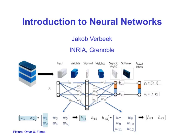
Jakob Verbeek INRIA, Grenoble
Picture: Omar U. Florez
Introduction to Neural Networks Jakob Verbeek INRIA, Grenoble - - PowerPoint PPT Presentation
Introduction to Neural Networks Jakob Verbeek INRIA, Grenoble Picture: Omar U. Florez Homework, Data Challenge, Exam All info at: http://lear.inrialpes.fr/people/mairal/teaching/2018-2019/MSIAM/ Exam (40%) Week Jan 28 Feb 1,
Picture: Omar U. Florez
All info at: http://lear.inrialpes.fr/people/mairal/teaching/2018-2019/MSIAM/
Exam (40%)
►
Week Jan 28 – Feb 1, 2019, duration 3h
►
Similar to homework
Homework (30%)
►
Can be done alone or in group of 2
►
Send to dexiong.chen@inria.fr
►
Deadline: Jan 7th, 2019
Data challenge (30%)
►
Can be done alone or in group of 2, not the same group as homework
►
Send report and code to dexiong.chen@inria.fr
►
Deadline Kaggle submission: Feb 11, 2019, Code+report Feb 13th
Neuron is basic computational unit of the brain
►
about 10^11 neurons in human brain
Simplified neuron model as linear threshold unit (McCulloch & Pitts, 1943)
►
Firing rate of electrical spikes modeled as continuous output quantity
►
Connection strength modeled by multiplicative weights
►
Cell activation given by sum of inputs
►
Output is non-linear function of activation
Basic component in neural circuits for complex tasks
Binary classification based on sign of generalized linear function
►
Weight vector w learned using special purpose machines
►
Fixed associative units in first layer, sign activation prevents learning
w
T ϕ (x)
sign (w
T ϕ(x))
ϕi(x)=sign (vT x)
20x20 pixel sensor Random wiring of associative units
Objective function linear in score over misclassified patterns
Perceptron learning via stochastic gradient descent
►
Eta is the learning rate
Potentiometers as weights adjusted by motors during learning
E(w)=−∑ti≠sign(f (xi)) ti f (xi)=∑i max (0,−t if (xi)) w
n+1=w n+η× tiϕ (xi) × [ti f (xi)<0]
ti∈{−1,+1}
If a correct solution w* exists, then the perceptron learning rule will converge to a correct solution in a finite number of iterations for any initial weight vector
Assume input lives in L2 ball of radius M, and without loss of generality that
►
w* has unit L2 norm
►
Some margin exists for the right solution
After a weight update we have
Moreover, since for misclassified sample, we have
Thus after t updates we have
Therefore , in limit of large t:
Since a(t) is upper bounded by construction by 1, the nr. of updates t must be limited.
For start at w=0, we have that
w '=w+ yx ⟨w
∗,w' ⟩=⟨w ∗,w⟩+ y ⟨w ∗, x⟩>⟨w ∗,w⟩+δ
y ⟨w
∗, x⟩>δ
⟨w' ,w' ⟩=⟨w ,w⟩+2 y⟨w , x⟩+⟨x , x⟩ <⟨w ,w⟩+⟨x , x⟩ <⟨w ,w⟩+M y ⟨w , x⟩<0 ⟨w
∗,w' ⟩>⟨w ∗,w⟩+t δ
⟨w' ,w' ⟩<⟨w ,w⟩+tM a(t)> δ
√M √t
a(t)= ⟨w
∗,w(t)⟩
√⟨w(t),w(t)⟩ > ⟨w
∗,w⟩+t δ
√⟨w ,w⟩+tM
t≤ M δ
2
Perceptron convergence theorem (Rosenblatt, 1962) states that
►
If training data is linearly separable, then learning algorithm finds a solution in a finite number of iterations
►
Faster convergence for larger margin
If training data is linearly separable then the found solution will depend on the initialization and ordering of data in the updates
If training data is not linearly separable, then the perceptron learning algorithm will not converge
No direct multi-class extension
No probabilistic output or confidence on classification
Perceptron loss similar to hinge loss without the notion of margin
►
Not a bound on the zero-one loss
►
Loss is zero for any separator, not only for large margin separators
All are either based on linear score function, or generalized linear function by relying on pre-defined non-linear data transformation or kernel f (x)=w
T ϕ (x)
Representer theorem states that in all these cases optimal weight vector is linear combination of training data
Kernel trick allows us to compute dot-products between (high-dimensional) embedding of the data
Classification function is linear in data representation given by kernel evaluations over the training data f (x)=w
T ϕ (x)=∑i αi⟨ϕ (xi),ϕ(x)⟩
w=∑i αiϕ (xi) k(xi , x)=⟨ϕ (xi),ϕ (x)⟩ f (x)=∑i αik(x , xi)=α
T k(x ,.)
Classification based on weighted “similarity” to training samples
►
Design of kernel based on domain knowledge and experimentation
►
Some kernels are data adaptive, for example the Fisher kernel
►
Still kernel is designed before and separately from classifier training
Number of free variables grows linearly in the size of the training data
►
Unless a finite dimensional explicit embedding is available
►
Can use kernel PCA to obtain such a explicit embedding
Alternatively: fix the number of “basis functions” in advance
►
Choose a family of non-linear basis functions
►
Learn the parameters of basis functions and linear function f (x)=∑i αik(x , xi)=α
T k(x ,.)
f (x)=∑i αiϕ i(x ;θi) ϕ (x)
Instead of using a generalized linear function, learn the features as well
Each unit in MLP computes
►
Linear function of features in previous layer
►
Followed by scalar non-linearity
Do not use the “step” non-linear activation function of original perceptron z j=h(∑i xi wij
(1))
z=h(W
(1)x)
yk=σ(∑j z jw jk
(2))
y=σ(W
(2)z)
Linear activation function leads to composition of linear functions
►
Remains a linear model, layers just induce a certain factorization
Two-layer MLP can uniformly approximate any continuous function on a compact input domain to arbitrary accuracy provided the network has a sufficiently large number of hidden units
►
Holds for many non-linearities, but not for polynomials
Consider simple case with D binary input units
►
Inputs and activations are all +1 or -1
►
Total number of possible inputs is 2D
►
Classification problem into two classes
Create hidden unit for each of M positive samples xm
►
Activation is +1 only if input equals xm
Let output implement an “or” over hidden units
MLP can separate any labeling over domain
►
But may need exponential number of hidden units to do so y=sign(∑m=1
M
zm+M−1) wm=xm zm=sign(wm
T x−D)
sign( y)={ +1 if y≥0 −1
MLP Architecture can be generalized
►
More than two layers of computation
►
Skip-connections from previous layers
Feed-forward nets are restricted to directed acyclic graphs of connections
►
Ensures that output can be computed from the input in a single feed- forward pass from the input to the output
Important issues in practice
►
Designing network architecture
Nr nodes, layers, non-linearities, etc
►
Learning the network parameters
Non-convex optimization
►
Sufficient training data
Data augmentation, synthesis
One output score for each target class
Multi-class logistic regression loss (cross-entropy loss)
►
Define probability of classes by softmax over scores
►
Maximize log-probability of correct class
As in logistic regression, but we are now learning the data representation concurrently with the linear classifier p(l=c∣x)= exp yc
Representation learning in discriminative and coherent manner
More generally, we can choose a loss function for the problem of interest and
this objective (regression, metric learning, ...) p(l=c∣x)= exp yc
L=−∑n ln p(ln∣xn)
1/(1+e
−x)
max(0, x) max (α x, x) max (w1
T x ,w2 T x)
nice interpretation as a saturating “firing rate” of a neuron
slide from: Fei-Fei Li & Andrej Karpathy & Justin Johnson
1. Saturated neurons “kill” the gradients, need activations to be exactly in right regime to obtain non-constant output 2. exp() is a bit compute expensive
[Nair & Hinton, 2010] slide from: Fei-Fei Li & Andrej Karpathy & Justin Johnson
[Mass et al., 2013] [He et al., 2015] slide from: Fei-Fei Li & Andrej Karpathy & Justin Johnson
[Goodfellow et al., 2013]
max(w1
T x ,w2 T x)
Non-convex optimization problem in general
►
Typically number of weights is very large (millions in vision applications)
►
Seems that many different local minima exist with similar quality
Regularization
►
L2 regularization: sum of squares of weights (“weight decay”)
►
“Drop-out”: deactivate random subset of neurons in each iteration
Similar to using many networks with less weights (shared among them)
►
Label smoothing: avoid overconfident, overfitted predictions
Training using gradient descend techniques
►
Stochastic gradient descend for large datasets (large N)
►
Estimate gradient by averaging over a relatively small number of samples 1 N ∑i=1
N
L(f (xi), yi;W )+λΩ(W ) L=(1−ϵ)log(p( y∣x))+ϵlog(1−p( y∣x))
Picture: Omar U. Florez
Forward propagation from input nodes to output nodes
►
Accumulate inputs via weighted sum into activation
►
Apply non-linear activation function f to compute output
Use Pre(j) to denote all nodes feeding into j a j=∑i∈Pre( j) wij xi x j=f (a j)
Node activation and output
Partial derivative of loss w.r.t. activation
Partial derivative w.r.t. learnable weights
Gradient of weight matrix between two layers given by outer-product of x and g g j= ∂ L ∂a j ∂ L ∂ wij = ∂ L ∂ a j ∂a j ∂wij =g j xi a j=∑i∈Pre( j) wij xi x j=f (a j) xi wij
Back-propagation layer-by-layer of gradient from loss to internal nodes
►
Application of chain-rule of derivatives
Accumulate gradients from downstream nodes
►
Post(i) denotes all nodes that i feeds into
►
Weights propagate gradient back
Multiply with derivative of local activation function gi=∂ xi ∂ai ∂ L ∂ xi =f ' (ai)∑ j∈Post (i) wij g j gi= ∂ L ∂ai a j=∑i∈Pre( j) wij xi x j=f (a j) ∂ L ∂ xi =∑ j∈Post(i) ∂ L ∂a j ∂a j ∂ xi =∑ j∈Post (i) g jwij
Special case for Rectified Linear Unit (ReLU) activations
Sub-gradient is step function
Sum gradients from downstream nodes
►
Set to zero if in ReLU zero-regime
►
Clip negative values in matrix vector product Wg
Gradient on incoming weights is “killed” by inactive units
►
Generates tendency for those units to remain inactive f (a)=max(0,a) f '(a)={ if a≤0 1
gi={ if ai≤0
∂ L ∂wij = ∂ L ∂a j ∂aj ∂ wij =g j xi
airplane automobile bird cat deer dog frog horse ship truck Input example : an image Output example: class label
How to represent the image at the network input?
A convolutional neural network is a special feedforward network
Hidden units are organized into grid, as is the input
Linear mapping from layer to layer takes form of convolution
►
Translation invariant processing
►
Local processing
►
Decouples nr of parameters from input size
►
Same net can process inputs of varying size
Fei-Fei Li & Andrej Karpathy & Justin Johnson
Lecture 7 - 27 Jan 2016
Preview: ConvNet is a sequence of Convolution Layers, interspersed with activation functions 32 32 3 28 slide from: Fei-Fei Li & Andrej Karpathy & Justin Johnson 28 6 CONV, ReLU e.g. 6 5x5x3 filters
Preview: ConvNet is a sequence of Convolutional Layers, interspersed with activation functions 32 32 3 CONV, ReLU e.g. 6 5x5x3 filters 28 28 6 CONV, ReLU e.g. 10 5x5x6 filters CONV, ReLU
10 24 24 slide from: Fei-Fei Li & Andrej Karpathy & Justin Johnson
Locally connected layer without weight sharing Convolutjonal layer used in CNN Fully connected layer as used in MLP
32 3
width height 32 depth slide from: Fei-Fei Li & Andrej Karpathy & Justin Johnson
32 32 3
Convolve the filter with the image i.e. “slide over the image spatially, computing dot products”
slide from: Fei-Fei Li & Andrej Karpathy & Justin Johnson
32 32 3
Convolve the filter with the image i.e. “slide over the image spatially, computing dot products”
slide from: Fei-Fei Li & Andrej Karpathy & Justin Johnson
32 32 3
slide from: Fei-Fei Li & Andrej Karpathy & Justin Johnson
T x+b
32 32 3
activation maps 1 28 28 convolve (slide) over all spatial locations
slide from: Fei-Fei Li & Andrej Karpathy & Justin Johnson
32 32 3
activation maps 1 28 28 convolve (slide) over all spatial locations
slide from: Fei-Fei Li & Andrej Karpathy & Justin Johnson
Fei-Fei Li & Andrej Karpathy & Justin Johnson
Lecture 7 - 27 Jan 2016
32 3 6 28 activation maps 32 28 Convolution Layer
For example, if we had 6 5x5 filters, we’ll get 6 separate activation maps: We stack these up to get a “new image” of size 28x28x6!
slide from: Fei-Fei Li & Andrej Karpathy & Justin Johnson
64 56 56 1x1 CONV with 32 filters 32 56 56 (each filter has size 1x1x64, and performs a 64-dimensional dot product) slide from: Fei-Fei Li & Andrej Karpathy & Justin Johnson
Applied separately per feature channel
Effect: invariance to small translations of the input
Max and average pooling most common, other things possible
►
Parameter free layer
►
Similar to strided convolution with special non-trainable filter
“Receptive field” is area in original image impacting a certain unit
►
Later layers can capture more complex patterns over larger areas
Receptive field size grows linearly over convolutional layers
►
If we use a convolutional filter of size w x w, then each layer the receptive field increases by (w-1)
Receptive field size increases exponentially over layers with striding
►
Regardless whether they do pooling or convolution
Convolutional and pooling layers typically followed by several “fully connected” (FC) layers, i.e. a standard MLP
►
FC layer connects all units in previous layer to all units in next layer
►
Assembles all local information into global vectorial representation
FC layers followed by softmax for classification
First FC layer that connects response map to vector has many parameters
►
Conv layer of size 16x16x256 with following FC layer with 4096 units leads to a connection with 256 million parameters !
►
Large 16x16 filter without padding gives 1x1 sized output map
then the signal shrinks as it passes through each layer untjl it’s too tjny to be useful.
then the signal grows as it passes through each layer untjl it’s too massive to be useful.
slide from: Fei-Fei Li & Andrej Karpathy & Justin Johnson
with standard deviatjon of sqrt(2/n), where n is the number of outputs to the neuron
same scale from one layer to the next
[Ioffe and Szegedy, 2015]
Initialization of NNs by explicitly forcing the activations throughout the network to take on a unit Gaussian distribution at the beginning
Normalization is a simple differentiable operation
“you want unit gaussian activations? just make them so.”
slide from: Fei-Fei Li & Andrej Karpathy & Justin Johnson
FC BN ReLU FC BN ...
slide from: Fei-Fei Li & Andrej Karpathy & Justin Johnson
ReLU
And then allow the network to squash the range if it wants to: Note, the network can learn: to recover the identity mapping. Normalize:
slide from: Fei-Fei Li & Andrej Karpathy & Justin Johnson
[Ioffe and Szegedy, 2015]
the network
vectors and their magnitude
activations, we can also normalize the weights to a similar effect [Salimans and Kingma, NIPS 2016] slide from: Fei-Fei Li & Andrej Karpathy & Justin Johnson
C1: 5x5 filters, outputs 6 channels, 156 = 6 (5x5 + 1) parameters
S2: “average” pooling, times constant + bias, 12 parameters
C3: 5x5 filters, outputs 16 channels, 1516 < 16 x 6 x (5x5 + 1) parameters
►
C3 features cannot see all S2 features
S4: “average” pooling, times constant + bias, 32 parameters
C5: 5x5 filters, outputs 120 channels, 49920 = 120 x16 (5x5 + 1) param.
F6: fully connected, 84 outputs, 10080 = 84 x 120 parameters
Final layer: 10 outputs, 840 = 84 x 10 parameters [LeCun, Bottou, Bengio, Haffner, Proceedings IEEE, 1998]
Large training datasets for computer vision
►
1.2 millions of 1000 classes in ImageNet challenge [Deng et al, CVPR’09]
►
200 million faces to train face recognition nets [Schroff et al., CVPR 2015]
GPU-based implementation: 1 to 2 orders of magnitude faster than CPU
►
Parallel computation for matrix products
►
Krizhevsky & Hinton, 2012: six days of training on two GPUs
►
Rapid progress in GPU compute performance
Network architectures
Industrially backed open-source software
►
Pytorch, TensorFlow, ...
Winner ImageNet 2012 image classification challenge, huge impact
►
CNNs improving “traditional” computer vision techniques on uncontrolled images, rather than datasets of small (eg 32x32) and controlled images
Compared to LeNet
►
Inputs at 224x224 rather than 32x32
►
Distributed implementation over 2 GPUs
►
5 rather than 3 conv layers
►
More feature channels in each layer
►
ReLU non-linearity
[Alex Krizhevsky & Geoff Hinton, NIPS 2012]
Double the number of layers 16 or 19 (from 8 in AlexNet)
Only small 3x3 filters, rather than filters up to size 11 AlexNet
►
Large filters approximated by sequence of smaller ones, receptive field increases, smaller nr of parameters due to factorization of weights
About 140 million parameters (AlexNet ~60 million) [Simonyan & Zisserman, ICLR ‘15] Winner ImageNet 2014 challenge
Reduced number of parameters: 5 million (60m AlexNet, 140m VGG)
Inception module: compress features before convolution
Replaces fully-connected layer with average pooling
Intermediate loss functions improve training of early layers
[Szegedy et al, CVPR 2015] Winner ImagetNet 2015 challenge
Figure: Kaiming He Fisher Vectors
More layers, smaller filters
ReLU non-linearity
Strided conv. rather than pooling
Dilation, up-down sampling
Residual and dense layer connectivity
Figure: Ferenc Huszár
Patches generating highest response for a selection of convolutional filters,
►
Showing 9 patches per filter
►
Zeiler and Fergus, ECCV 2014
Layer 1: simple edges and color detectors
Layer 2: corners, center-surround, ...
Layer 3: various object parts
Layer 4+5: selective units for entire objects or large parts of them
Early CNN layers extract generic features that seem useful for different tasks
►
Object localization, semantic segmentation, action recognition, etc.
On some datasets too little training data to learn CNN from scratch
►
For example, only few hundred objects bounding box to learn from
Pre-train AlexNet/VGGnet/ResNet/DenseNet on large scale dataset
►
In practice mostly ImageNet classification: millions of labeled images
►
Also works with noisy image tags from Flickr [Joulin et al. ECCV 2016]
Fine-tune CNN weights for task at hand, possibly with modifed architecture
►
Replace classification layer, add bounding box regression, …
►
Reduced learning rate and possibly freezing early network layers
Object category localization
Semantic segmentation
Task: given an image report a tight bounding box around every instance of an
►
For example detect all people, sheep, dogs, … in an image
Problem formulation: scoring hypothetical object locations
►
Avoid strong overlap between hypothesis with non-maximum suppression
►
Threshold on score to decide on number of objects
Instance Segmentation
Classify each possible dection window as being a tight bounding box for a pedestrian, car, sheep, …
►
Sliding window: translate windows of given size & aspect ratio over image
►
Crop detection window from image, feed to CNN image classifier
Unreasonably many image regions to consider if applied in naive manner
►
Tremendous cost to evaluate CNN at many positions
Solutions 1) Use a smaller set of windows at plausible positions 2) Share computations across different windows 3) Do more than classification: bounding box regression R-CNN, Girshick et al., CVPR 2014
Many methods exist, some data driven learning based method
[Alexe et al. 2010, Zitnick & Dollar 2014, Cheng et al. 2014]
Selective search method [Sande et al. ICCV’11, Uijlings et al. IJCV’13]
► Unsupervised multi-resolution hierarchical segmentation ► Detections proposals generated as bounding box of segments ► 1500 windows per image suffice to cover over 95% of true objects
with sufficient accuracy
Naively applying CNN across many cropped or warped windows is wasteful
►
At window overlap convolutions are computed multiple times
Instead: compute convolutional layers only once across entire image
►
Pool features using max-pooling into fixed-size representation
►
Fully connected layers up to classification computed per window
Speedup in practice about 2 orders of magnitude [He et al. ECCV 2014, Girshick ICCV’15]
Classification CNN only extracts a single scalar from every image window
Additionally: predict the offset of the true object location with respect to the candidate detection window
►
Optionally for several “anchor” boxes [Ren et al. ICCV’15]
Region proposal network returns regressed bounding boxes
►
Pool convolutional features across these boxes
►
Classify the regressed box with more CNN layers (regress again)
RoI’s are again processed independently
[Picture from Leonardo Araujo dos Santos]
Region proposal network directly returns regressed bounding boxes
Detect anchor boxes at different scales and from different network layers
Using K different “anchor” boxes, each layer of WxH activations outputs KxWxH regressed bounding boxes with corresponding scores
No further per-box processing after regression: speedup [Liu et al. ECCV’16]
Object category localization
Semantic segmentation
Task: given an image assign every pixel to a category
►
For example: background, person, sheep, dog, etc
Problem formulation: classify pixels independently from each other
►
Extract patch centered on pixel of interest, feed to classification CNN
►
Possibly ensure spatial consistency in post-processing step
Instance Segmentation
Assign each pixel to an object or background category
►
Consider running CNN on small image patch to determine its category
►
Train by optimizing per-pixel classification loss
Want to avoid wasteful computation of convolutional filters
►
Compute convolutional layers once per image
►
Here all local image patches are at the same scale
►
Many more local regions: dense, at every pixel Long et al., CVPR 2015
Interpret fully connected layers as 1x1 sized convolutions
►
Function of features in previous layer, but only at own position
►
Still same function is applied across all positions
Five sub-sampling layers reduce the resolution of output map by factor 32
Up-sampling via bi-linear interpolation gives blurry predictions
Alternative shift input image by few pixels, but requires 32x32 CNN evaluations to get output for each pixel...
Combine response maps at different resolutions
►
Upsampling of the later and coarser layers, concatenate with finer layers Long et al., CVPR 2015
Simplest form: use bilinear interpolation or nearest neighbor interpolation
►
Note that these can be seen as upsampling by zero-padding, followed by convolution with specific filters, no channel interactions
Idea can be generalized by learning the convolutional filter
►
No need to hand-pick the interpolation scheme
►
Can include channel interactions, if those turn out be useful
Resolution-increasing counterpart of strided convolution
►
Similarly, average and max pooling can be written in terms of convolutions [Saxena & Verbeek, NIPS 2016]
Results obtained using skip-connections from earlier layers
Detail better preserved when using finer resolutions
Filter size and number of parameters are normally coupled
For fixed filter size, large field of view can be obtained by
►
More layers using a fixed filter: slow growth
►
Down sampling the signal: looses resolution
Dilated convolution (“filtre à trous”): Large filter with many zeros
►
Large field of view without loosing resolution
Decoupling field-of-view and the number of parameters in a filter
[Yu & Koltun, ICLR ‘16]
Similar to strided convolutions, but keeping full resolution in result
►
Can result in aliasing effect due to subsampling of high resolution features
High-resolution layers are memory intensive
►
4x more activations as compared to each factor 2 downsampling
►
Limits the number of feature channels that can be used
Receptive field of repeated 2-dilated convolutional layers
[Ronneberger et al. 2015]
Combines ideas of skip connections and conv-deconv architecture
►
Skip connections to maintain high-resolution signal
►
Progressive upsampling from coarse to fine
Beyond independent prediction of pixel labels
Conditional random fields (CRF): encourage nearby and similar pixels to take the same label value
Efficient inference for fully connected CRFs (all pixel pairs are connected
[Krahenbuhl & Koltun, NIPS’11]
Integrate CRF model within CNN training [Zheng et al.,
ICCV’15]
Classification CNN goes from full-res input to 1x1 classification signal
►
Chain of convolution and pooling layers from input to output
Dense prediction problems require high resolution and large field-of-view
►
Semantic segmentation, object localization, optical flow prediction, etc
What are the right architectures?
►
Filter sizes, positioning of convolutions vs pooling, type of pooling, etc
►
Are chain-structured networks the best for classification ?
[Saxena & Verbeek, NIPS 2016]
Grid of network layers across multiple scales
►
Feed-forward across the horizontal “layer axis”
►
Nothing new in training: standard back-prop gradient calculation
Chain-structured networks (eg for classification) and other networks (such as Unet for segmentation) are special cases of this more general structure
[Saxena & Verbeek, NIPS 2016]
Each feature map receives input from three others
►
Scale finer: strided convolution
►
Scale coarser: stride coarse activations on finer resolution, then covolution
►
Same scale: standard convolution
Generalizes very large class of networks with “standard” layers
With enough layers and feature channels, 3x3 convolutions suffice for
►
Average pooling, max-pooling, and strided convolition
►
Nearest-neighbor, bi-linear, and general deconvolution up-sampling
►
Filters of any size by distribution over layers
[Saxena & Verbeek, NIPS 2016]
Connection strengths in a fabric learned for image classification
Weak connections may be suppressed
►
CIFAR-10: reduce nr. of connections by factor 3, error up from 7.4% to 8.1%
Search over cost effective networks can be integrated in training
[Veniat & Denoyer, arXiv’17]
[Fourure et al, BMVC 2017]
Grid of network layers across multiple scales
►
Feed-forward and residual across the horizontal “layer axis”
Down-sampling block followed by up-sampling block
Accuracy close to state of the art (similar to FRRN), trained “from scratch”
►
Few thousand training images, instead of pre-trained ImageNet classification
[Huang et al, arXiv 2017]
Grid of network layers across multiple scales
►
Feed-forward and dense connections across the horizontal “layer axis”
Down-sampling across all layers for classification
Intermediate classifiers for any-time prediction
[Huang et al, arXiv 2017]
Efficient any-time prediction model
►
Features computed for early classifiers are re-used for later classifiers