Introduction to Machine Learning k -Nearest Neighbors Regression - - PowerPoint PPT Presentation

introduction to machine learning k nearest neighbors
SMART_READER_LITE
LIVE PREVIEW

Introduction to Machine Learning k -Nearest Neighbors Regression - - PowerPoint PPT Presentation

Introduction to Machine Learning k -Nearest Neighbors Regression Learning goals Understand the basic idea of k-NN Know different distance measures for different scales of feature variables Understand that k-NN has no optimization step


slide-1
SLIDE 1

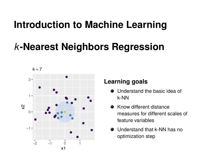
Introduction to Machine Learning k-Nearest Neighbors Regression

Learning goals

Understand the basic idea of k-NN Know different distance measures for different scales of feature variables Understand that k-NN has no

  • ptimization step
slide-2
SLIDE 2

NEAREST NEIGHBORS: INTUITION

Say we know locations of cities in 2 different countries. Say we know which city is in which country. Say we don’t know where the countries’ border is. For a given location, we want to figure out which country it belongs to. Nearest neighbor rule: every location belongs to the same country as the closest city. k-nearest neighbor rule: vote over the k closest cities (smoother)

c

  • Introduction to Machine Learning – 1 / 13
slide-3
SLIDE 3

K-NEAREST-NEIGHBORS

k-NN can be used for regression and classification It generates predictions ˆ y for a given x by comparing the k

  • bservations that are closest to x

"Closeness" requires a distance or similarity measure (usually: Euclidean). The set containing the k closest points x(i) to x in the training data is called the k-neighborhood Nk(x) of x.

−1 1 2 −2 −1 1

x1 x2 k = 15

−1 1 2 −2 −1 1

x1 x2 k = 7

−1 1 2 −2 −1 1

x1 x2 k = 3 c

  • Introduction to Machine Learning – 2 / 13
slide-4
SLIDE 4

DISTANCE MEASURES

How to calculate distances? Most popular distance measure for numerical features: Euclidean distance Imagine two data points x = (x1, ..., xp) and ˜ x = (˜ x1, ..., ˜ xp) with p features ∈ R The Euclidean distance: dEuclidean (x, ˜ x) =

  • p
  • j=1

(xj − ˜

xj)2

c

  • Introduction to Machine Learning – 3 / 13
slide-5
SLIDE 5

DISTANCE MEASURES

Example: Three data points with two metric features each: a = (1, 3), b = (4, 5) and c = (7, 8) Which is the nearest neighbor of b in terms of the Euclidean distance? d(b, a) =

  • (4 − 1)2 + (5 − 3)2 = 3.61

d(b, c) =

  • (4 − 7)2 + (5 − 8)2 = 4.24

⇒ a is the nearest neighbor for b.

Alternative distance measures are: Manhattan distance dmanhattan(x, ˜ x) =

p

  • j=1

|xj − ˜

xj| Mahalanobis distance (takes covariances in X into account)

c

  • Introduction to Machine Learning – 4 / 13
slide-6
SLIDE 6

DISTANCE MEASURES

Comparison between Euclidean and Manhattan distance measures:

1 2 3 4 5 6 1 2 3 4 5 Dimension 1 Dimension 2 x x ~ Manhattan Euclidean d(x, x ~) = |5−1| + |4−1| = 7 d( x , x ~) = ( 5 − 1)2 +( 4 − 1)2 = 5

c

  • Introduction to Machine Learning – 5 / 13
slide-7
SLIDE 7

DISTANCE MEASURES

Categorical variables, missing data and mixed space: The Gower distance dgower(x, ˜ x) is a weighted mean of dgower(xj, ˜ xj): dgower(x, ˜ x) =

p

  • j=1

δxj,˜

xj · dgower(xj, ˜

xj)

p

  • j=1

δxj,˜

xj

. δxj,˜

xj is 0 or 1. It becomes 0 when the j-th variable is missing in at

least one of the observations (x or ˜ x), or when the variable is asymmetric binary (where “1” is more important/distinctive than “0”, e. g., “1” means “color-blind”) and both values are zero. Otherwise it is 1.

c

  • Introduction to Machine Learning – 6 / 13
slide-8
SLIDE 8

DISTANCE MEASURES

dgower(xj, ˜ xj), the j-th variable contribution to the total distance, is a distance between the values of xj and ˜

  • xj. For nominal variables the

distance is 0 if both values are equal and 1 otherwise. The contribution of other variables is the absolute difference of both values, divided by the total range of that variable.

c

  • Introduction to Machine Learning – 7 / 13
slide-9
SLIDE 9

DISTANCE MEASURES

Example of Gower distance with data on sex and income:

index sex salary 1 m 2340 2 w 2100 3 NA 2680

dgower(x, ˜ x) =

p

  • j=1

δxj ,˜

xj ·dgower(xj,˜

xj)

p

  • j=1

δxj ,˜

xj

dgower(x(1), x(2)) =

1·1+1· |2340−2100|

|2680−2100|

1+1

=

1+ 240

580

2

= 1+0.414

2

= 0.707

dgower(x(1), x(3)) =

0·1+1· |2340−2680|

|2680−2100|

0+1

=

0+ 340

580

1

= 0+0.586

1

= 0.586

dgower(x(2), x(3)) =

0·1+1· |2100−2680|

|2680−2100|

0+1

=

0+ 580

580

1

= 0+1.000

1

= 1

c

  • Introduction to Machine Learning – 8 / 13
slide-10
SLIDE 10

DISTANCE MEASURES

Weights: Weights can be used to address two problems in distance calculation: Standardization: Two features may have values with a different

  • scale. Many distance formulas (not Gower) would place a higher

importance on a feature with higher values, leading to an

  • imbalance. Assigning a higher weight to the lower-valued feature

can combat this effect. Importance: Sometimes one feature has a higher importance (e. g., more recent measurement). Assigning weights according to the importance of the feature can align the distance measure with known feature importance. For example: dweighted

Euclidean (x, ˜

x) =

  • p
  • j=1

wj(xj − ˜ xj)2

c

  • Introduction to Machine Learning – 9 / 13
slide-11
SLIDE 11

K-NN REGRESSION

Predictions for regression:

ˆ

y = 1 k

  • i:x(i)∈Nk(x)

y(i)

ˆ

y = 1

  • i:x(i)∈Nk(x) wi
  • i:x(i)∈Nk(x)

wiy(i) with neighbors weighted according to their distance to x: wi =

1 d(x(i),x)

c

  • Introduction to Machine Learning – 10 / 13
slide-12
SLIDE 12

K-NN SUMMARY

k-NN has no optimization step and is a very local model. We cannot simply use least-squares loss on the training data for picking k, because we would always pick k = 1. k-NN makes no assumptions about the underlying data distribution. The smaller k, the less stable, less smooth and more “wiggly” the decision boundary becomes. Accuracy of k-NN can be severely degraded by the presence of noisy or irrelevant features, or when the feature scales are not consistent with their importance.

c

  • Introduction to Machine Learning – 11 / 13
slide-13
SLIDE 13

K-NN SUMMARY

Hypothesis Space: Step functions over tesselations of X . Hyperparameters: distance measure d(·, ·) on X ; size of neighborhood k. Risk: Use any loss function for regression or classification. Optimization: Not applicable/necessary. But: clever look-up methods & data structures to avoid computing all n distances for generating predictions.

c

  • Introduction to Machine Learning – 12 / 13