c i j
play

c i,j max k,m c k,m 4 Wednesday, 2 Oct. 2019 Machine Learning - PowerPoint PPT Presentation

Uses of Nearest Neighbors } Once we have found the k -nearest neighbors of a point, we can use this information: In and of itself : sometimes we just want to know what 1. those nearest neighbors actually are (items that are similar to a given


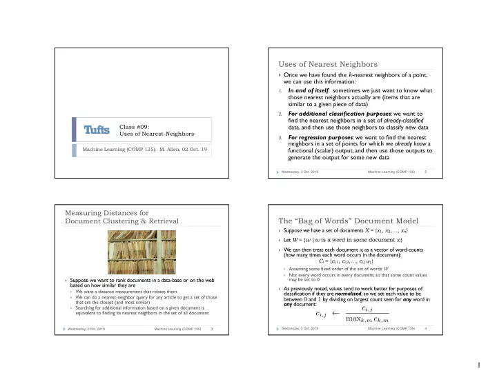
  1. Uses of Nearest Neighbors } Once we have found the k -nearest neighbors of a point, we can use this information: In and of itself : sometimes we just want to know what 1. those nearest neighbors actually are (items that are similar to a given piece of data) For additional classification purposes : we want to 2. find the nearest neighbors in a set of already-classified Class #09: data, and then use those neighbors to classify new data Uses of Nearest-Neighbors For regression purposes : we want to find the nearest 3. neighbors in a set of points for which we already know a Machine Learning (COMP 135): M. Allen, 02 Oct. 19 functional (scalar) output, and then use those outputs to generate the output for some new data 2 Wednesday, 2 Oct. 2019 Machine Learning (COMP 135) Measuring Distances for The “Bag of Words” Document Model Document Clustering & Retrieval } Suppose we have a set of documents X = { x 1 , x 2 ,…, x n } } Let W = { w | w is a word in some document x i } } We can then treat each document x i as a vector of word-counts (how many times each word occurs in the document): C i = { c i, 1 , c i, 2 ,…, c i, | W | } } Assuming some fixed order of the set of words W } Not every word occurs in every document, so that some count values may be set to 0 } Suppose we want to rank documents in a data-base or on the web based on how similar they are } As previously noted, values tend to work better for purposes of } We want a distance measurement that relates them classification if they are normalized , so we set each value to be } We can do a nearest-neighbor query for any article to get a set of those between 0 and 1 by dividing on largest count seen for any word in that are the closest (and most similar) any document: } Searching for additional information based on a given document is c i,j equivalent to finding its nearest neighbors in the set of all document c i,j ← max k,m c k,m 4 Wednesday, 2 Oct. 2019 Machine Learning (COMP 135) 3 Wednesday, 2 Oct. 2019 Machine Learning (COMP 135) 1

  2. <latexit sha1_base64="9AlSyY3dNL6afTRkAF6okxiuCqU=">ACiHicZVFNa9wEJXdr8T92rTHXIbutmwhbG03kORQCMmlxS62UC8GK0sb0Rky0j2MH41/T/9J5/E63XPbgZkBhG72ZeVoVUhj0/QfHfb8xctXO7ve6zdv370f7X24NKrUjM+ZkpfrajhUuR8jgIlvyo0p9lK8sXq9nzvrj2giV/8b7gi8zus5FKhFW4pHf1hcT6uv8OUHRMhrbKIxoMi4gUrpBCbVBRjpTYgckgUKzOeI0zqSQtR5EW6lLzxC2ybILS3xyKDOq47uYzWcVNBZImLFvo+Q1LYkXBaHdTbEVJNWbOFtk0v1sajsT/zu4CnSdAnY9LHRTz6G/0blUlqzHVguy0bqlEwyVsvKg0vKLula950Frbw2ZYSJW2xy7YVQe4XGFn2YB9XWJ6vGxEXpTIc7aVSUsJqGDjNiRCc4by3iaUaWH7A7uhdkm0fzJQ2piSHMDd5iMTO6tcK4u/yUI7rzUg+H/dp8lOAu+z8Jfh+PTs96KHbJPpEpCcgROSU/yQWZE+bsOt+cY+fE9VzfPXJPtlDX6TkfySDcs0dGBsDG</latexit> Distances between Words Better Measures of Document Similarity We want to emphasize rare words over common ones: } We can now compute the distance function between any } Define word frequency: t(w,x) as the (normalized) count of occurrences of word 1. two documents (here we use the Euclidean): w in document x v c x ( w ) = # times word w occurs in document x | W | u u X d ( x i , x j ) = ( c i,k − c j,k ) 2 t c ? x = max w ∈ W c x ( w ) k =1 t ( w, x ) = c x ( w ) } We could then build a KD-Tree, using the vectors of c ? x words as our dimension values, and query for some set of Define inverse document frequency of word w : 2. most similar documents to any document we start with Total # of | X | documents id ( w ) = log } Problem : word counts turn out to be a lousy metric! 1 + |{ x ∈ X | w ∈ x }| # that contain word w } Common every-day words dominate the counts, making most Use combined measure for each word and document: 3. documents appear quite similar, and making retrieval poor tid ( w, x ) = t ( w, x ) × id ( w ) 6 Wednesday, 2 Oct. 2019 Machine Learning (COMP 135) 5 Wednesday, 2 Oct. 2019 Machine Learning (COMP 135) Inverse Document Frequency An Example } The inverse document frequency of word w : } We want to emphasize rare words over common ones: | X | id ( w ) = log | X | 1 + |{ x ∈ X | w ∈ x }| id ( w ) = log } Suppose we have 1,000 documents ( | X | = 1000 ), and the word 1 + |{ x ∈ X | w ∈ x }| the occurs in every single one of them: id ( the ) = log 1000 tid ( w, x ) = t ( w, x ) × id ( w ) 1001 ≈ − 0 . 001442 } Conversely, if the word banana only appears in 10 of them: } id ( w ) goes to 0 as the word w becomes more common id ( banana ) = log 1000 ≈ 6 . 644 } tid ( w,x ) is highest when w occurs often in document x , but 10 is rare overall in the full document set } Thus, when calculating normalized word-counts, banana gets treated as being about 4,600 times more important than the ! } If we threshold id ( w ) to a minimum of 0 (never negative) we then completely ignore words that are in every document 8 Wednesday, 2 Oct. 2019 Machine Learning (COMP 135) 7 Wednesday, 2 Oct. 2019 Machine Learning (COMP 135) 2

  3. <latexit sha1_base64="RNW3oSmy0/Xtc0SYqhDUtdbRE=">ADC3icnVJLb9NAEF6bVwmPpnDksiIqiqUS2Wml9lKpKheORSJNpWxqbdabdJO1+yO+5Dlf1D+DNygV67c+TesHaPW5IDESLuancf3zc7MJXCgO/ctx79x8fLT2uPXk6bPn6+2NF8dGZrxAVNS6ZMJNVyKhA9AgOQnqeY0nkg+nCzelf7hOdGqOQjXKV8HNZIqaCUbCmcMPZjLqXodjCl+Hcw2/2MTGfNOTEZHGYL/aD4jQnjOoHxYF7oKIuhfhowWHn6L7znfaLzAhLaIzyXM/hSLfLu/Wv1BHcAeUgIi5wUtgb2xJbt3zFXfF+V+kNcIfwEYN9mO3lBVH2O74Pb8SvKoEtdJBtRyF7Z8kUiyLeQJMUmNGga1qnFMNgkletEhmeErZgs54Xk2xwJvWFOGp0vYkgCtrIy5RUE2tkT3KYLo3zkWSZsATtoSZhKDwuXAcSQ0ZyCvrEKZFpYfszOqKQO7Fg2ksoXRFj4vdymytcqZsvFncd/WaxsQ/P3dVeW43wu2e/0PO52Dw7oVa+gVeo26KEC76AC9R0dogJhz7Xxvjs37mf3q/vNvVmGuk6d8xI1xP3xGzHQ8EY=</latexit> Nearest-Neighbor Clustering Image source: Hastie, et al., Elements of Distances between Words for Image Classification Statistical Learning (Springer, 2017) Given the threshold on the inverse document frequency, the distance between two } Spectral Band 1 Spectral Band 2 Spectral Band 3 documents is now proportional to that measure: v | W | u u X d ( x i , x j ) = ( tid ( w k , x i ) − tid ( w k , x j )) 2 t k =1 v | W | u Spectral Band 4 Land Usage Predicted Land Usage u X = ([ t ( w k , x i ) × id ( w k )] − [ t ( w k , x j ) × id ( w k )]) 2 t k =1 v | W | u u X ( id ( w k ) × [ t ( w k , x i ) − t ( w k , x j )]) 2 = t k =1 } The STATLOG project (Michie et al., 1994): given satellite imagery of land, predict its agricultural use for mapping purposes Our KD-T ree can now efficiently find similar documents based upon this metric } Mathematically, words for which frequency id ( w ) = 0 have no effect on the distance } } T raining set: sets of images in 4 spectral bands, with actual use of Obviously, in implementing this we can simply remove those words from word-set W in the first land (7 soil/crop categories) based upon manual survey } place to skip useless clock-cycles… 10 Wednesday, 2 Oct. 2019 Machine Learning (COMP 135) 9 Wednesday, 2 Oct. 2019 Machine Learning (COMP 135) Nearest-Neighbor Clustering Image source: Hastie, et al., Elements of Nearest-Neighbor Regression for Image Classification Statistical Learning (Springer, 2017) } Given a data-set of various Spectral Band 1 Spectral Band 2 Spectral Band 3 features of abalone (sex, size, weight, etc.), a regression N N N classifier predicts shellfish age N X N } A training set of Spectral Band 4 Land Usage Predicted Land Usage measurements, with real age N N N determined by counting rings in the abalone shell, is analyzed and grouped into nearest neighbor units } T o predict the usage for a given pixel in a new image: In each band, get value of a pixel and 8 adjacent, for (4 x 9) = 36 features 1. } A predictor for new data is Find the 5 nearest neighbors of that feature-vector in labeled training set 2. generated according to the Assign the land use class of the majority of those 5 neighbors 3. average age value of neighbors } Achieved test error of 9.5% with a very simple algorithm 12 Wednesday, 2 Oct. 2019 Machine Learning (COMP 135) 11 Wednesday, 2 Oct. 2019 Machine Learning (COMP 135) 3

  4. Nearest-Neighbor Regression This Week & Next 1-nearest neighbor 5-nearest neighbors } T oday : Nearest Neighbors, Clustering and Regression } Next : Support Vector Machines } Readings : Linked from class website schedule page. } Homework 02 : due Thursday, 03 October, 9:00 AM } Homework 03 : due Wednesday, 16 October, 9:00 AM } Predictions for 100 points, given regression on shell length and age } Office Hours : 237 Halligan, Tuesday, 11:00 AM – 1:00 PM } With one-nearest neighbor (left), the result has higher variability and } TA hours can be found on class website as well predictions are noisier } With five-nearest neighbors (right), results are smoothed out over multiple data-points 14 Wednesday, 2 Oct. 2019 Machine Learning (COMP 135) 13 Wednesday, 2 Oct. 2019 Machine Learning (COMP 135) 4
Download Presentation
Download Policy: The content available on the website is offered to you 'AS IS' for your personal information and use only. It cannot be commercialized, licensed, or distributed on other websites without prior consent from the author. To download a presentation, simply click this link. If you encounter any difficulties during the download process, it's possible that the publisher has removed the file from their server.

Recommend


More recommend